Analyze Relation Between Parameters and Design Requirements

To analyze how the parameters and states (collectively referred to as parameters) of a Simulink^® model influence the design requirement on the model signals, you first generate samples of the parameters. You then define the cost function by creating a design requirement on the model signals, and evaluate the cost function for each sample. Finally, you analyze the relationship between the parameter variations and the cost function values. You can perform this analysis in the following ways:

Visual Analysis

View a plot of the cost function evaluations against the parameter samples to identify trends. This method is informal and provides visual intuition about how the various parameters affect the cost function.

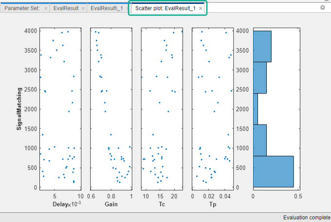
In the Sensitivity Analyzer, after the evaluation is complete, an evaluation result scatter plot is generated in the app. The plot displays the evaluated cost function value as a function of each parameter in the parameter set. The last column subplot displays the probability distribution of the evaluated cost function values. You can add a best-fit line to the scatter subplots by right-clicking in the plot, and selecting Overlay linear fit in the context menu. In this plot, the best-fit line indicates that the Gain parameter has a lot of influence on the requirement.

Evaluation Result scatter plot

You can also plot a contour plot of the evaluated results. To learn more about these plots, see Interact with Plots in the Sensitivity Analyzer. For an example, see Identify Key Parameters for Estimation (GUI).

At the command line, you can use tools such as:

sdo.scatterPlot — Scatter plot of the parameter samples against the cost function evaluation
surf, mesh, contour — 3-D plot of samples of two parameters against the cost function evaluation

For an example, see Identify Key Parameters for Estimation (Code).

Statistical Analysis

In addition to visually analyzing the effect of parameters on the cost function, you can also compute statistics to quantify the relation.

Obtain summary statistics about the relationship between cost function evaluations and parameters samples. Available analysis methods include:

Method	Description
Correlation	Use to analyze how a model parameter and the cost function output are correlated.
Partial Correlation	Use to analyze how a model parameter and the cost function are correlated, removing the effects of the remaining parameters.
Standardized Regression	Use when you expect that the model parameters linearly influence the cost function.

For each of these methods, you specify what data to use for the analysis by choosing from the following analysis types:

Linear analysis, also referred to as Pearson analysis — Uses raw data for analysis. Use linear analysis when you expect a linear relation between the parameters and cost function, and when the residuals about the best-fit line are expected to be normally distributed. Linear analysis is also recommended when the number of samples, and so the number of residual points is large.
Ranked analysis, also referred to as Spearman analysis and ranked transformation — Uses ranks of data for analysis. Use ranked analysis when you expect a nonlinear monotonic relation between the parameters and the cost function and when the residuals about the best-fit line are not normally distributed. Ranked analysis is also recommended when the number of samples, and so the number of residual points is small.
Linear analysis retains information about intervals between data values, whereas ranked analysis does not. Suppose that you had the following data set:
x₁ x₂ y
9 20 340
5 60 106
2.3 50.4 870.5
Here x₁ and x₂ are model parameters, and y is the cost function. Each row represents a sample and the associated cost function evaluation.
The data is ranked on a per column basis. For example, when you rank the data in column 1 (x₁), which contains the entries 9, 5, and 2.3, the ranked data is equal to 3, 2, and 1. The ranked data set for the samples of x₁, x₂ and y are as follows:
x₁ x₂ y
3 1 2
2 3 1
1 2 3
The ranked data set can be used for correlation, partial correlation, or standardized regression analysis.
Kendall — Kendall’s tau rank correlation coefficient is calculated.
Applicable when the analysis method is Correlation. Requires Statistics and Machine Learning Toolbox™ software.

x₁	x₂	y
9	20	340
5	60	106
2.3	50.4	870.5

x₁	x₂	y
3	1	2
2	3	1
1	2	3

Correlation Method

Calculates the correlation coefficients, R. Use this method to analyze how a model parameter and the cost function outputs are correlated.

R is calculated as follows:

$\begin{array}{l} R (i, j) & = \frac{C (i, j)}{\sqrt{C (i, i) C (j, j)}} \\ C & = c o v (x, y) \\ = E [(x - μ_{x}) (y - μ_{y})] \\ μ_{x} & = E [x] \\ μ_{y} & = E [y] \end{array}$

x contains Ns samples of Np model parameters. y contains Ns rows, each row corresponds to the cost function evaluation for a sample in x.

R values are in the [-1 1] range. The (i,j) entry of R indicates the correlation between x(i) and y(j).

R(i,j) > 0 — Variables have positive correlation. The variables increase together.
R(i,j) = 0 — Variables have no correlation.
R(i,j) < 0 — Variables have negative correlation. As one variable increases, the other decreases.

Partial Correlation Method

Calculates the partial correlation coefficients, R. This method requires Statistics and Machine Learning Toolbox software. Use this method to analyze how a model parameter and the cost function are correlated, adjusting to remove the effect of the other parameters.

R is calculated using partialcorri (Statistics and Machine Learning Toolbox) from the Statistics and Machine Learning Toolbox software.

Standardized Regression Method

Calculates the standardized regression coefficients, R. Use this method when you expect that the model parameters linearly influence the cost function.

R is calculated as follows:

$R = b_{x} \frac{σ_{x}}{σ_{y}}$

Consider a single sample (x₁,...,xNp) and the corresponding single output, y. b_x is the regression coefficient vector calculated using least squares assuming a linear model $\hat{y} = b_{0} + \sum_{i = 1}^{N p} {\hat{b}}_{x_{i}} x_{i}$ . R standardizes each element of b_x by multiplying it with the ratio of the standard deviation of the corresponding x sample (σ_x) to the standard deviation of y (σ_y).

Perform Statistical Analysis

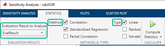
In the Sensitivity Analyzer, after you have evaluated the design requirements, specify the analysis methods and types in the Statistics tab of the app.

Select the evaluation results you want to analyze in the Evaluation Result to Analyze list. After that, you specify the analysis methods and types, and click Compute Statistics. You can compute all applicable combinations of analysis methods and types.

Evaluation Result to Analyze, Method, and Type are highlighted on the statistics tab of the app

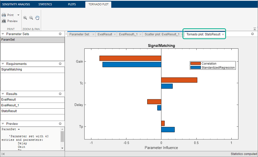
The results of the analysis are returned in the StatsResult variable, in the Results area of the app. In this case, the StatsResult variable includes the linear (Pearson) correlation coefficients and linear standardized regression coefficients calculated between the cost function and each parameter. To see the coefficients, right-click StatsResult, and select Open in the context-menu.

A tornado plot is generated that displays the results of the analysis in order of influence of parameters on the cost function. The parameter that most influences the cost function is displayed on the top. As was seen in the results scatter plot, in this tornado plot the Gain parameter has the most influence on the design requirement cost function.

Tornado plot of StatsResult

To learn more about tornado plots, see Interact with Plots in the Sensitivity Analyzer. For an example, see Identify Key Parameters for Estimation (GUI).

At the command line, specify the analysis methods and types using sdo.analyze. This function performs linear correlation analysis by default. To specify other analysis methods, use sdo.AnalyzeOptions. For an example, see Identify Key Parameters for Estimation (Code).