Main Content

Luenberger Observer

Discrete-time Luenberger observer

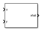
  • Luenberger Observer block

Libraries:
Simscape / Electrical / Control / Observers

Description

The Luenberger Observer block implements a discrete time Luenberger observer. Use this block to estimate the states of an observable system using:

  • The discrete inputs and outputs of the system.

  • A discrete state-space representation of the system.

The Luenberger Observer is also sometimes referred to as a state observer or simply an observer.

You can control multi-input, multi-output systems by passing the output state vector of this block to a State Feedback Controller block.

Defining Equations

The block implements a discrete time Luenberger Observer using the backward Euler method due to its simplicity and stability.

The estimator is given by this difference equation:

x^(k+1) =Adx^(k) +Bdu(k) + Ld(y(k) y^(k)),

where:

  • x^(k) is the kth estimated state vector.

  • y^(k) is the kth estimated output vector.

  • u(k) is the kth input vector.

  • y(k) is the kth measured output vector.

  • Ad is the discretized state matrix.

  • Bd is the discretized input matrix.

  • Ld is the discretized observer gain matrix.

The dynamics of the estimation error are described by:

e(k+1)=(AdLdCd)e(k),

where:

  • e(k) is the kth error vector.

  • Cd is the output matrix.

The estimation error converges to zero when Ad-LdCd has its eigenvalues inside the unit circle. Therefore, the value of Ld should be such that this goal is achieved. The block computes the observer gain by solving

LdT=GX1,

where G is an arbitrary matrix and X is obtained by solving the Sylvester equation:

AdTXXΛ=CdTG.

Here, Λ is a matrix with the desired eigenvalues, which are not the same as the eigenvalues of Ad. This diagram shows the basic structure of a discrete time Luenberger Observer.

Assumptions

The system is observable, which is true if the state of the system can be determined from the input and output in a finite time. Mathematically, this means that the system observability matrix has full rank.

Limitations

The desired eigenvalues are not the same as the eigenvalues of the open-loop model.

Examples

Ports

Input

expand all

Input signal to the system whose state we want to estimate, specified as a vector.

Data Types: single | double

Measured output of the system whose state we want to estimate, specified as a vector.

Data Types: single | double

Output

expand all

Estimate of the state of the system, specified as a vector.

Data Types: single | double

Parameters

expand all

Select the strategy for parameterizing the state-space matrices and desired poles for the observer. The block implementation is discrete regardless of this parameterization.

State matrix of the discrete-time state-space model. The A matrix must be square, with the number of rows and columns equal to the order of the system.

Dependencies

To enable this parameter, set State-space parameterization to Discrete-time.

Input matrix of the discrete-time state-space model. The B matrix must have the number of rows equal to the order of the system, and the number of columns equal to the number of system inputs.

Dependencies

To enable this parameter, set State-space parameterization to Discrete-time.

Output matrix of the discrete-time state-space model. The C matrix must have the number of rows equal the number of outputs of the system, and the number of columns equal to the order of the system.

Dependencies

To enable this parameter, set State-space parameterization to Discrete-time.

Feedthrough matrix of the discrete-time state-space model. The D matrix must have the number of rows equal to the number of system outputs, and the number of columns equal to the number of system inputs.

Dependencies

To enable this parameter, set State-space parameterization to Discrete-time.

State matrix of the continuous-time state-space model. The A matrix must be square, with the number of rows and columns equal to the order of the system.

Dependencies

To enable this parameter, set State-space parameterization to Continuous-time.

Input matrix of the continuous-time state-space model. The B matrix must have the number of rows equal to the order of the system, and the number of columns equal to the number of system inputs.

Dependencies

To enable this parameter, set State-space parameterization to Continuous-time.

Output matrix of the continuous-time state-space model. The C matrix must have the number of rows equal the number of outputs of the system, and the number of columns equal to the order of the system.

Dependencies

To enable this parameter, set State-space parameterization to Continuous-time.

Feedthrough matrix of the continuous-time state-space model. The D matrix must have the number of rows equal to the number of system outputs, and the number of columns equal to the number of system inputs.

Dependencies

To enable this parameter, set State-space parameterization to Continuous-time.

Select the strategy for parameterizing observer gain.

Dependencies

To enable this parameter, set State-space parameterization to Discrete-time.

Specify the observer gain that puts all eigenvalues of the matrix Ad-LdCd inside the unit circle. The gain matrix must have the number of rows equal to number of system inputs and the number of columns equal to the order of the system.

Dependencies

To enable this parameter, set:

  • State-space parameterization to Discrete-time.

  • Observer design to Observer gain.

Specify the location of the eigenvalues:

  • To have negative real part if State-space parameterization is set to Continuous-time. In this case, the eigenvalues of the continuous-time system are approximated to the discrete ones based on the Discretization sample time.

  • To lie within the unit circle if State-space parameterization is set to Discrete-time.

The Observer gain is then calculated based on these eigenvalues. The size of the vector should be the same as the system order.

Select the initial condition of each state.

Value used to discretize the state space matrices and also approximate the discrete-time eigenvalues.

Dependencies

To enable this parameter, set State-space parameterization to Continuous-time.

Value used to simulate the dynamics of the model. Choose the same value as Discretization sample time, unless the block is placed within a triggered subsystem, in which case you must set it to -1.

References

[1] Luenberger, D. G. "An Introduction to Observers." IEEE Transactions on Automatic Control. Vol. 16, Number 6, 1971, pp. 596-602.

[2] Alessandri, A., and P. Coletta. "Design of Luenberger observers for a class of hybrid linear systems." In International Workshop on Hybrid Systems: Computation and Control, Berlin, March 2001.

[3] Varga, A. "Robust pole assignment via Sylvester equation based state feedback parametrization." In Computer-Aided Control System Design, pp. 13-18., Anchorage, Alaska, 2000.

Extended Capabilities

C/C++ Code Generation
Generate C and C++ code using Simulink® Coder™.

Version History

Introduced in R2017b