Test Difficult-to-Reproduce Chart Configurations

This example shows how to use operating points to test how a chart responds to a combination of active states and data values that is difficult to reproduce during simulation. An operating point is a snapshot of the state of a Simulink^® model during simulation. If your model contains a Stateflow^® chart, the operating point includes information about active states, output and local data, and persistent variables. For more information, see Save and Restore Operating Points for Stateflow Charts.

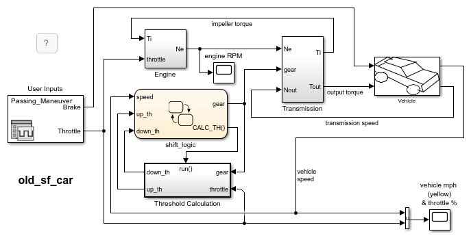
The model old_sf_car illustrates a four-speed automatic transmission system of a car.

Model old_sf_car.

In this model, the Stateflow chart shift_logic implements the logic for shifting between four gears. The substates of the parallel state gear_shift represent the gears in the transmission system. The entry actions in these substates set the value of the chart output gear. As a result, during normal simulation, the value of gear reflects which substate is active.

Stateflow chart shift_logic.

By default, the model simulates for 30 seconds.

Scope showing simulation results between t=0 and t=30.

To see what happens when the value of the chart output gear changes abruptly, simulate the model, save the operating point at t = 10, modify the operating point to reflect a change in the chart output, and then simulate again between t = 10 and t = 30.

Define Operating Point for Initial Segment

Open the model old_sf_car.
```
openExample("old_sf_car")
```
Set the model to save the final operating point. Open the Configuration Parameters dialog box and, in the Data Import/Export pane:
1. Select Final states and enter a name for the operating point. For this example, use xSteadyState.
2. Select Save final operating point.
3. Click OK.
Set the stop time for this simulation segment. In the Simulation tab, set Stop Time to 10.
Run the simulation.
When you simulate the model, you save the final operating point at t = 10 in the variable xSteadyState in the MATLAB^® base workspace. At t = 10, the engine operates at a steady-state value of 2500 RPM.
In the Configuration Parameters dialog box, in the Data Import/Export pane, clear the Save final operating point and Final states parameters. This step prevents you from overwriting the operating point you saved in the previous step.

Modify Operating Point for Change in Data Value

Access the Stateflow.op.BlockOperatingPoint object that contains the operating point information for the shift_logic chart.

blockpath = "old_sf_car/shift_logic";
op = get(xSteadyState,blockpath)

op = 

Block:    "shift_logic"    (handle)    (active)
  Path:     old_sf_car/shift_logic

  Contains:

    + gear_state         "State (AND)"          (active)
    + selection_state    "State (AND)"          (active)
      gear               "Block output data"    double [1, 1]

The operating point contains a list of states and data in hierarchical order.

Highlight the states that are active in the chart at t = 10.
```
highlightActiveStates(op)
```
Active states appear highlighted. The transmission system is in a steady state in fourth gear.

Access the Stateflow.op.OperatingPointData object that contains the operating point information for the chart output gear.

op.gear

ans = 

      Description: 'Block output data'
         DataType: 'double'
             Size: '[1, 1]'
            Range: [1x1 struct]
     InitialValue: [1x0 double]
            Value: 4

Change the value of gear to 1.
```
op.gear.Value = 1;
```

Save the modified operating point.

xModified = set(xSteadyState,blockpath,op);

Test Model Behavior after Change in Data Value

Load the operating point as the initial state of the model. In the Configuration Parameters dialog box, in the Data Import/Export pane, select Initial state and enter the variable that contains the modified operating point of your chart, xModified. Then, click OK.
Define the stop time for the simulation segment to test. In the Simulation tab, set Stop Time to 30.
Run the simulation.
The chart animation shows that the system continually attempts to compensate for the high vehicle speed relative to the chart output gear by shifting up, but is unable to because the system is already in fourth gear.
As a result, the engine RPM increases to 6000 RPM.