bootstrp

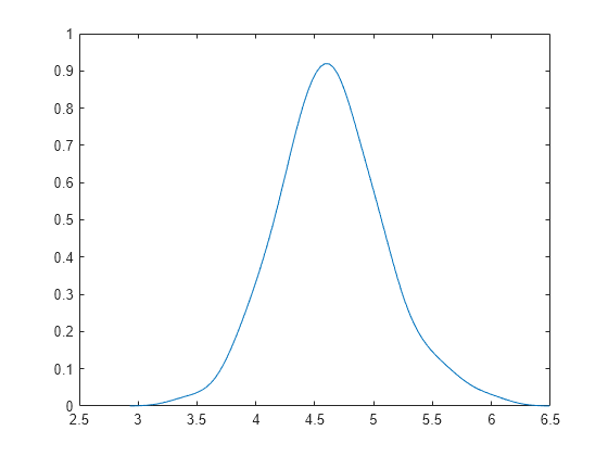
Estimate the kernel density of bootstrapped means.

Generate 100 random numbers from the exponential distribution with mean 5.

rng('default')  % For reproducibility
y = exprnd(5,100,1);

Compute a sample of 100 bootstrapped means of random samples taken from the vector y.

m = bootstrp(100,@mean,y);

Plot an estimate of the density of the bootstrapped means.

[fi,xi] = ksdensity(m);
plot(xi,fi)

Compute and plot the means and standard deviations of 100 bootstrap samples.

Generate 100 random numbers from the exponential distribution with mean 5.

rng('default')  % For reproducibility
y = exprnd(5,100,1);

Compute a sample of 100 bootstrapped means and standard deviations of random samples taken from the vector y.

stats = bootstrp(100,@(x)[mean(x) std(x)],y);

Plot the bootstrap estimate pairs.

plot(stats(:,1),stats(:,2),'o')
xlabel('Mean')
ylabel('Standard Deviation')

Take bootstrap samples of patient data, compute the mean measurements for each data sample, and visualize the results.

Load the patients data set. Create the matrix patientData containing age, weight, and height measurements. Each row of patientData corresponds to one patient.

load patients
patientData = [Age Weight Height];

Create 200 bootstrap data samples from the data in patientData. To create each sample, randomly select with replacement 100 rows (that is, size(patientData,1)) from the rows in patientData. For each sample, calculate the mean age, weight, and height measurements. Each row of bootstat contains the three mean measurements for one bootstrap sample.

rng('default') % For reproducibility
bootstat = bootstrp(200,@mean,patientData);

Visualize the mean measurements for all 200 bootstrap data samples. Note that bootstrap samples with greater mean weights tend to have greater mean heights.

scatter3(bootstat(:,1),bootstat(:,2),bootstat(:,3))
xlabel('Mean Age')
ylabel('Mean Weight')
zlabel('Mean Height')

view([-75 10])

Compute a correlation coefficient standard error using bootstrap resampling of the sample data.

Load the lawdata data set, which contains the LSAT score and law school GPA for 15 students.

load lawdata
rng('default')  % For reproducibility
size(lsat)

ans = 1×2

    15     1

size(gpa)

ans = 1×2

    15     1

Create 1000 data samples by resampling the 15 data points, and compute the correlation between the two variables for each data sample.

[bootstat,bootsam] = bootstrp(1000,@corr,lsat,gpa);

Display the first 5 bootstrapped correlation coefficients.

bootstat(1:5,:)

ans = 5×1

    0.9874
    0.4918
    0.5459
    0.8458
    0.8959

Display the indices of the data selected for the first 5 bootstrap samples.

bootsam(:,1:5)

ans = 15×5

    13     3    11     8    12
    14     7     1     7     4
     2    14     5    10     8
    14    12     1    11    11
    10    15     2    12    14
     2    10    13     5    15
     5     1    11    11     9
     9    13     5    10     3
    15    15    15     3     3
    15    11     1     2     4
      ⋮

Create a histogram that shows the variation of the correlation coefficient across all the bootstrap samples.

histogram(bootstat)

The sample minimum is positive, indicating that the relationship between LSAT score and GPA is not accidental.

Finally, compute a bootstrap standard of error for the estimated correlation coefficient.

se = std(bootstat)

se = 
0.1285

Compare bootstrap samples with different observation weights. Create a custom function that computes statistics for each sample.

Create 50 bootstrap samples from the numbers 1 through 6. To create each sample, bootstrp randomly chooses with replacement from the numbers 1 through 6, six times. This process is similar to rolling a die six times. For each sample, the custom function countfun (shown at the end of this example) counts the number of 1s in the sample.

rng('default') %For reproducibility
counts = bootstrp(50,@countfun,(1:6)');

Note: If you use the live script file for this example, the countfun function is already included at the end of the file. Otherwise, you need to create this function at the end of your .m file or add it as a file on the MATLAB® path.

Create 50 bootstrap samples from the numbers 1 through 6, but assign different weights to the numbers. Each time bootstrp randomly chooses from the numbers 1 through 6, the probability of choosing a 1 is 0.5, the probability of choosing a 2 is 0.1, and so on. Again, countfun counts the number of 1s in each sample.

weights = [0.5 0.1 0.1 0.1 0.1 0.1]';
weightedCounts = bootstrp(50,@countfun,(1:6)','Weights',weights);

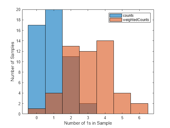
Compare the two sets of bootstrap samples by using histograms.

histogram(counts)
hold on
histogram(weightedCounts)
legend
xlabel('Number of 1s in Sample')
ylabel('Number of Samples')
hold off

The two sets of bootstrap samples have different distributions; in particular, the samples in the second set tend to contain more 1s. For example, of the 50 samples in the first set, only two samples contain more than two 1s. By contrast, of the 50 samples in the second set (with observation weights), $$12+14+4+2=32$$ samples contain more than two 1s.

This code creates the function countfun.

function numberofones = countfun(sample)
numberofones = sum(sample == 1);
end

Estimate the standard errors for a coefficient vector in a linear regression by bootstrapping the residuals.

Note: This example uses regress, which is useful when you simply need the coefficient estimates or residuals of a regression model and you need to repeat fitting a model multiple times, as in the case of bootstrapping. If you need to investigate a fitted regression model further, create a linear regression model object by using fitlm.

Load the sample data.

load hald

Perform a linear regression, and compute the residuals.

x = [ones(size(heat)),ingredients];
y = heat;
b = regress(y,x);
yfit = x*b;
resid = y - yfit;

Estimate the standard errors by bootstrapping the residuals.

se = std(bootstrp(1000,@(bootr)regress(yfit+bootr,x),resid))

se = 1×5

   56.1752    0.5940    0.5815    0.5989    0.5691