Bootstrap Aggregation (Bagging) of Classification Trees Using TreeBagger

Statistics and Machine Learning Toolbox™ offers two objects that support bootstrap aggregation (bagging) of classification trees: TreeBagger created by using TreeBagger and ClassificationBaggedEnsemble created by using fitcensemble. See Comparison of TreeBagger and Bagged Ensembles for differences between TreeBagger and ClassificationBaggedEnsemble.

This example shows the workflow for classification using the features in TreeBagger only.

Use ionosphere data with 351 observations and 34 real-valued predictors. The response variable is categorical with two levels:

The goal is to predict good or bad returns using a set of 34 measurements.

Fix the initial random seed, grow 50 trees, inspect how the ensemble error changes with accumulation of trees, and estimate feature importance. For classification, it is best to set the minimal leaf size to 1 and select the square root of the total number of features for each decision split at random. These settings are defaults for TreeBagger used for classification.

load ionosphere
rng(1945,'twister')
b = TreeBagger(50,X,Y,'OOBPredictorImportance','On');
figure
plot(oobError(b))
xlabel('Number of Grown Trees')
ylabel('Out-of-Bag Classification Error')

The method trains ensembles with few trees on observations that are in bag for all trees. For such observations, it is impossible to compute the true out-of-bag prediction, and TreeBagger returns the most probable class for classification and the sample mean for regression. You can change the default value returned for in-bag observations using the DefaultYfit property. If you set the default value to an empty character vector for classification, the method excludes in-bag observations from computation of the out-of-bag error. In this case, the curve is more variable when the number of trees is small, either because some observations are never out of bag (and are therefore excluded) or because their predictions are based on few trees.

b.DefaultYfit = '';
figure
plot(oobError(b))
xlabel('Number of Grown Trees')
ylabel('Out-of-Bag Error Excluding In-Bag Observations')

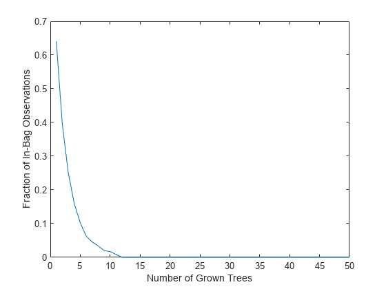
The OOBIndices property of TreeBagger tracks which observations are out of bag for what trees. Using this property, you can monitor the fraction of observations in the training data that are in bag for all trees. The curve starts at approximately 2/3, which is the fraction of unique observations selected by one bootstrap replica, and goes down to 0 at approximately 10 trees.

finbag = zeros(1,b.NumTrees);
for t=1:b.NTrees
    finbag(t) = sum(all(~b.OOBIndices(:,1:t),2));
end
finbag = finbag / size(X,1);
figure
plot(finbag)
xlabel('Number of Grown Trees')
ylabel('Fraction of In-Bag Observations')

Estimate feature importance.

figure
bar(b.OOBPermutedPredictorDeltaError)
xlabel('Feature Index')
ylabel('Out-of-Bag Feature Importance')

Select the features yielding an importance measure greater than 0.75. This threshold is chosen arbitrarily.

idxvar = find(b.OOBPermutedPredictorDeltaError>0.75)

idxvar = 1×5

     3     5     7     8    27

Having selected the most important features, grow a larger ensemble on the reduced feature set. Save time by not permuting out-of-bag observations to obtain new estimates of feature importance for the reduced feature set (set OOBVarImp to 'off'). You would still be interested in obtaining out-of-bag estimates of classification error (set OOBPred to 'on').

b5v = TreeBagger(100,X(:,idxvar),Y,'OOBPredictorImportance','off','OOBPrediction','on');
figure
plot(oobError(b5v))
xlabel('Number of Grown Trees')
ylabel('Out-of-Bag Classification Error')

For classification ensembles, in addition to classification error (fraction of misclassified observations), you can also monitor the average classification margin. For each observation, the margin is defined as the difference between the score for the true class and the maximal score for other classes predicted by this tree. The cumulative classification margin uses the scores averaged over all trees and the mean cumulative classification margin is the cumulative margin averaged over all observations. The oobMeanMargin method with the 'mode' argument set to 'cumulative' (default) shows how the mean cumulative margin changes as the ensemble grows: every new element in the returned array represents the cumulative margin obtained by including a new tree in the ensemble. If training is successful, you would expect to see a gradual increase in the mean classification margin.

The method trains ensembles with few trees on observations that are in bag for all trees. For such observations, it is impossible to compute the true out-of-bag prediction, and TreeBagger returns the most probable class for classification and the sample mean for regression.

For decision trees, a classification score is the probability of observing an instance of this class in this tree leaf. For example, if the leaf of a grown decision tree has five 'good' and three 'bad' training observations in it, the scores returned by this decision tree for any observation fallen on this leaf are 5/8 for the 'good' class and 3/8 for the 'bad' class. These probabilities are called 'scores' for consistency with other classifiers that might not have an obvious interpretation for numeric values of returned predictions.

figure
plot(oobMeanMargin(b5v));
xlabel('Number of Grown Trees')
ylabel('Out-of-Bag Mean Classification Margin')

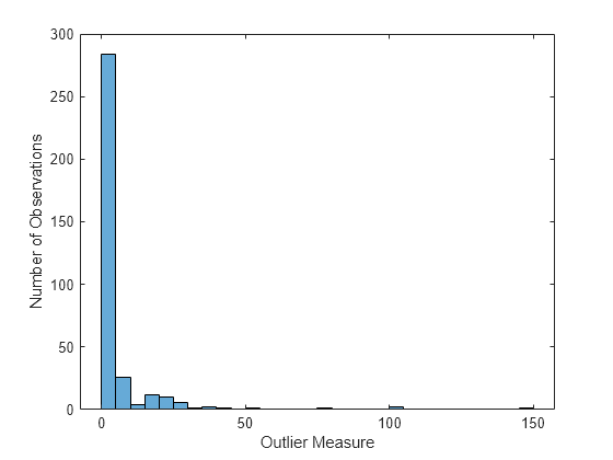
Compute the matrix of proximities and examine the distribution of outlier measures. Unlike regression, outlier measures for classification ensembles are computed within each class separately.

b5v = fillProximities(b5v);
figure
histogram(b5v.OutlierMeasure)
xlabel('Outlier Measure')
ylabel('Number of Observations')

Find the class of the extreme outliers.

extremeOutliers = b5v.Y(b5v.OutlierMeasure>40)

extremeOutliers = 6x1 cell
    {'g'}
    {'g'}
    {'g'}
    {'g'}
    {'g'}
    {'g'}

percentGood = 100*sum(strcmp(extremeOutliers,'g'))/numel(extremeOutliers)

percentGood = 
100

All of the extreme outliers are labeled 'good'.

As for regression, you can plot scaled coordinates, displaying the two classes in different colors using the 'Colors' name-value pair argument of mdsProx. This argument takes a character vector in which every character represents a color. The software does not rank class names. Therefore, it is best practice to determine the position of the classes in the ClassNames property of the ensemble.

gPosition = find(strcmp('g',b5v.ClassNames))

gPosition = 
2

The 'bad' class is first and the 'good' class is second. Display scaled coordinates using red for the 'bad' class and blue for the 'good' class observations.

figure
[s,e] = mdsProx(b5v,'Colors','rb');
xlabel('First Scaled Coordinate')
ylabel('Second Scaled Coordinate')

Plot the first 20 eigenvalues obtained by scaling. The first eigenvalue clearly dominates and the first scaled coordinate is most important.

figure
bar(e(1:20))
xlabel('Scaled Coordinate Index')
ylabel('Eigenvalue')

Another way of exploring the performance of a classification ensemble is to plot its receiver operating characteristic (ROC) curve or another performance curve suitable for the current problem. Obtain predictions for out-of-bag observations. For a classification ensemble, the oobPredict method returns a cell array of classification labels as the first output argument and a numeric array of scores as the second output argument. The returned array of scores has two columns, one for each class. In this case, the first column is for the 'bad' class and the second column is for the 'good' class. One column in the score matrix is redundant because the scores represent class probabilities in tree leaves and by definition add up to 1.

[Yfit,Sfit] = oobPredict(b5v);

Use rocmetrics to compute a performance curve. By default, rocmetrics computes true positive rates and false positive rates for a ROC curve.

rocObj = rocmetrics(b5v.Y,Sfit(:,gPosition),'g');

Plot the ROC curve for the 'good' class by using the plot function of rocmetrics.

plot(rocObj)

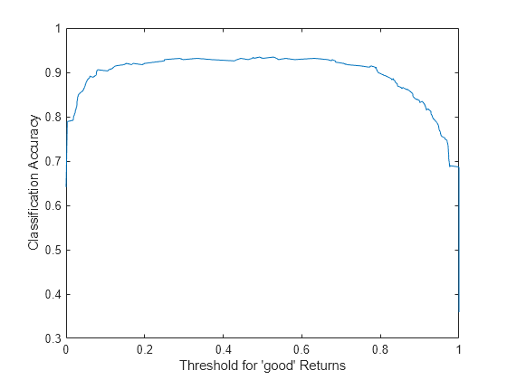
Instead of the standard ROC curve, you might want to plot, for example, ensemble accuracy versus threshold on the score for the 'good' class. Compute accuracy by using the addMetrics function of rocmetrics. Accuracy is the fraction of correctly classified observations, or equivalently, 1 minus the classification error.

rocObj = addMetrics(rocObj,'Accuracy');

Create a plot of ensemble accuracy versus threshold.

thre = rocObj.Metrics.Threshold;
accu = rocObj.Metrics.Accuracy;
plot(thre,accu)
xlabel('Threshold for ''good'' Returns')
ylabel('Classification Accuracy')

The curve shows a flat region indicating that any threshold from 0.2 to 0.6 is a reasonable choice. By default, a classification model assigns classification labels using 0.5 as the boundary between the two classes. You can find exactly what accuracy this corresponds to.

[~,idx] = min(abs(thre-0.5));
accu(idx)

ans = 
0.9316

Find the maximal accuracy.

[maxaccu,iaccu] = max(accu)

maxaccu = 
0.9345

iaccu = 
99

The maximal accuracy is a little higher than the default one. The optimal threshold is therefore.

thre(iaccu)

ans = 
0.5278

See Also

TreeBagger | compact | oobError | mdsprox | oobMeanMargin | oobPredict | perfcurve | fitcensemble

Related Topics

• Bootstrap Aggregation (Bagging) of Regression Trees Using TreeBagger
• Comparison of TreeBagger and Bagged Ensembles
• Use Parallel Processing for Regression TreeBagger Workflow