Compare Linear Regression Models Using Regression Learner App
This example shows how to compare a linear regression model and an efficiently trained
linear regression model using the Regression Learner app. Efficiently trained linear
regression models are useful for performing linear regression with many observations and
many predictors. For large in-memory data, efficient linear regression models that use
fitrlinear tend to train and predict faster
than linear regression models that use fitlm. Export the efficient linear regression model to the workspace and
inspect its properties, such as its size and linear coefficients. Then, use the model to
make predictions on new data.
Note that you can use efficient linear regression models with smaller data sets. If necessary, adjust the relative coefficient tolerance (beta tolerance) to improve the fit. The default value is sometimes too large for the app to converge to a good model. For more information, see Efficiently Trained Linear Model Hyperparameter Options.
In the MATLAB® Command Window, simulate 10,000 observations from the model y = x100 + 2x200 + e, where X = x1, …, x1000 is a 10,000-by-1000 matrix with 10% nonzero standard normal elements, and e is a vector of random normal errors with mean 0 and standard deviation 0.3.
rng("default") % For reproducibility
X = full(sprandn(10000,1000,0.1));
y = X(:,100) + 2*X(:,200) + 0.3*randn(10000,1);
Open the Regression Learner app.
regressionLearner
On the Learn tab, in the File section, click New Session and select From Workspace Data.
In the New Session from Workspace Data dialog box, select the matrix
Xfrom the Data Set Variable list. Then, under Response, click the From workspace option button and selectyfrom the list.To accept the default validation scheme and continue, click Start Session. The default validation option is 5-fold cross-validation, to protect against overfitting.
The app creates a plot of the response with the record number on the x-axis.
Create a selection of linear models. On the Learn tab, in the Models section, click the arrow to open the gallery. In the Linear Regression Models group, click Linear.
Reopen the gallery and click Efficient Linear Least Squares in the Efficiently Trained Linear Regression Models group.
In the Models pane, delete the draft fine tree model by right-clicking it and selecting Delete.
On the Learn tab, in the Train section, click Train All and select Train All.
Note
If you have Parallel Computing Toolbox™, then the Use Parallel button is selected by default. After you click Train All and select Train All or Train Selected, the app opens a parallel pool of workers. During this time, you cannot interact with the software. After the pool opens, you can continue to interact with the app while models train in parallel.
If you do not have Parallel Computing Toolbox, then the Use Background Training check box in the Train All menu is selected by default. After you select an option to train models, the app opens a background pool. After the pool opens, you can continue to interact with the app while models train in the background.
Regression Learner trains the two linear models. In the Models pane, the app outlines the RMSE (Validation) (root mean squared error) of the best model.
Compare the two models. On the Learn tab, in the Plots and Results section, click Layout and select Compare models.
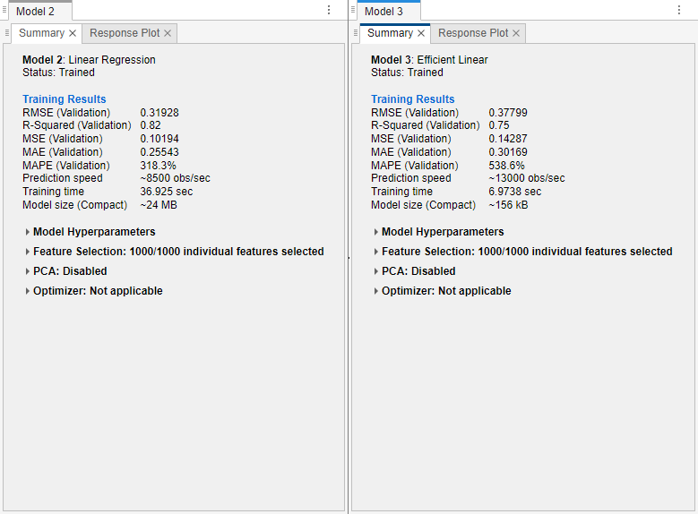
Click the Summary tab for each model.
Note
Validation introduces some randomness into the results. Your model validation results might vary from the results shown in this example.
The validation RMSE for the linear regression model (Model 2) is better than the validation RMSE of the efficient linear model (Model 3). However, the training time for the efficient linear model is significantly smaller than the training time for the linear regression model. Also, the estimated model size of the efficient linear model is significantly smaller than the size of the linear regression model.
For each model, plot the predicted response versus the true response. On the Learn tab, in the Plots and Results section, click the arrow to open the gallery, and then click Predicted vs. Actual (Validation) in the Validation Results group. Use this plot to determine how well the regression model makes predictions for different response values.
Click the Hide plot options button
 at the top right of the plots to make more
room for the plots.
at the top right of the plots to make more
room for the plots.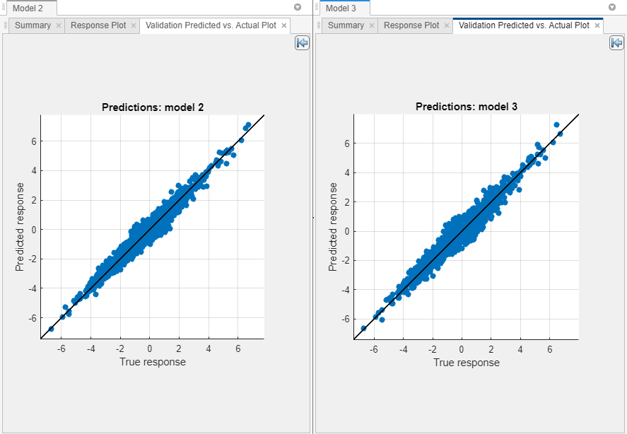
A perfect regression model has predicted responses equal to the true responses, so all the points lie on a diagonal line. The vertical distance from the line to any point is the error of the prediction for that point. A good model has small errors, so the predictions are scattered near the line. Typically, a good model has points scattered roughly symmetrically around the diagonal line.
In this example, both models perform well.
For each model, view the residuals plot. On the Learn tab, in the Plots and Results section, click the arrow to open the gallery, and then click Residuals (Validation) in the Validation Results group. The residuals plot displays the difference between the predicted and true responses.
Click the Hide plot options button
at the top right of the plots to make more
room for the plots.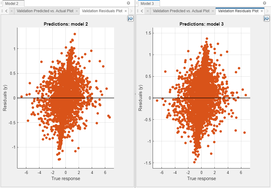
Typically, a good model has residuals scattered roughly symmetrically around 0. If you can see any clear patterns in the residuals, you can most likely improve your model.
In this example, the models have similar residual distributions.
Because the efficient linear model performs similarly to the linear regression model, export a compact version of the efficiently trained linear regression model to the workspace. In the Export section of the Learn tab, click Export and select Export Model to Workspace. In the Export Regression Model dialog box, the check box to include the training data is disabled because efficient linear models do not store training data. In the dialog box, click OK to accept the default variable name.
In the MATLAB workspace, extract the
RegressionLinearmodel from thetrainedModelstructure. Inspect the size of the trained modelMdl.Mdl = trainedModel.RegressionEfficientLinear; whos MdlNote that you can extract the model from the exported structure because Regression Learner did not use a feature transformation or feature selection technique to train the model.Name Size Bytes Class Attributes Mdl 1x1 159411 RegressionLinear
Plot the linear coefficients from the efficient linear model.
coefficients = Mdl.Beta;
plot(coefficients,".")
xlabel("Predictor")
ylabel("Coefficient")
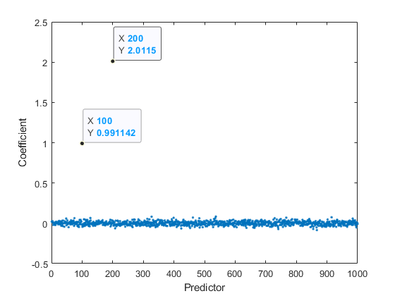
The coefficient for the 100th predictor is approximately 1, the coefficient for the 200th predictor is approximately 2, and the remaining coefficients are close to 0. These values match the coefficients of the model used to generate the simulated training data.
Use the model to make predictions on new data. For example, create a 50-by-1000 matrix with 10% nonzero standard normal elements. You can use either the
predictFcnfunction of thetrainedModelstructure or thepredictobject function of theMdlobject to predict the response for the new data. These two methods are equivalent because Regression Learner did not use a feature transformation or feature selection technique to train the model.XTest = full(sprandn(50,1000,0.1)); predictedY1 = trainedModel.predictFcn(XTest); predictedY2 = predict(Mdl,XTest); isequal(predictedY1,predictedY2)
If the exportedans = logical 1
trainedModelcontains PCA or feature selection information, use thepredictFcnfunction of the structure to predict on new data.