glyphplot

Visualize multidimensional data by using a star plot. Notice how the stars differ across the observations.

Load the fisheriris data set, which contains four measurements (sepal length, sepal width, petal length, and petal width) from three species of iris flowers.

load fisheriris

The matrix meas contains all four measurements for 150 flowers. Display the measurements for the first eight flowers.

head(meas)

    5.1000    3.5000    1.4000    0.2000
    4.9000    3.0000    1.4000    0.2000
    4.7000    3.2000    1.3000    0.2000
    4.6000    3.1000    1.5000    0.2000
    5.0000    3.6000    1.4000    0.2000
    5.4000    3.9000    1.7000    0.4000
    4.6000    3.4000    1.4000    0.3000
    5.0000    3.4000    1.5000    0.2000

Create a glyph plot using the iris measurements in meas. By default, glyphplot creates a star plot and standardizes the measurements before plotting.

glyphplot(meas)
title("Glyph Plots for Iris Data")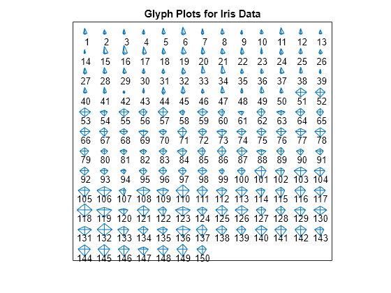

Each star corresponds to an iris, and each spoke corresponds to one of the standardized iris measurements. The length of a spoke indicates the relative value of the measurement.

Notice that the first 50 flowers tend to have smaller stars than the next 50 flowers. Similarly, both of those sets of flowers tend to have smaller stars than the last 50 flowers.

Compare the distribution of the measurements for the three sets of irises by using box plots.

figure
boxchart(meas(1:50,:))
hold on
boxchart(meas(51:100,:))
boxchart(meas(101:end,:))
hold off
legend(["Irises 1-50","Irises 51-100","Irises 101-150"])
xticklabels(["Sepal Length","Sepal Width","Petal Length","Petal Width"])
title("Box Plots for Iris Data")

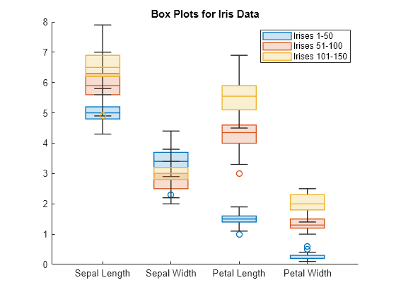
The box plots show that, for three of the four measurements, the first 50 irises tend to have smaller values than the next 50 irises, and those irises tend to have smaller values than the last 50 irises. Because smaller values correspond to shorter star spokes, this result helps explain the relative size of the stars in the previous star plot.

Visualize multidimensional data by using a Chernoff face plot. Specify the facial features corresponding to the data variables.

Load the carsmall data set, which contains measurements for 100 cars. Combine the Acceleration, Displacement, Horsepower, MPG, and Weight variables into a table. Display the values for the first 12 cars.

load carsmall
Tbl = table(Acceleration,Displacement,Horsepower,MPG,Weight);
head(Tbl,12)

    Acceleration    Displacement    Horsepower    MPG    Weight
    ____________    ____________    __________    ___    ______

          12            307            130         18     3504 
        11.5            350            165         15     3693 
          11            318            150         18     3436 
          12            304            150         16     3433 
        10.5            302            140         17     3449 
          10            429            198         15     4341 
           9            454            220         14     4354 
         8.5            440            215         14     4312 
          10            455            225         14     4425 
         8.5            390            190         15     3850 
        17.5            133            115        NaN     3090 
        11.5            350            165        NaN     4142 

Create a Chernoff face plot using the car measurements in Tbl. Note that glyphplot excludes observations with missing values from the plot and, by default, standardizes the car measurements before plotting.

glyphplot(Tbl{:,:},Glyph="face")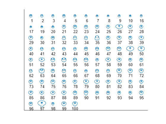

By default, glyphplot uses the face size to represent the first variable (in this case, Acceleration). The forehead-to-jaw relative arc length represents the second variable (Displacement), the forehead shape represents the third variable (Horsepower), the jaw shape represents the fourth variable (MPG), and the width between the eyes represents the fifth variable (Weight). For more information, see Facial Features.

Change the previous plot so that the MPG variable is not displayed and the jaw shape represents the Weight variable instead.

figure
glyphplot(Tbl{:,:},Glyph="face",Features=[1 2 3 0 4])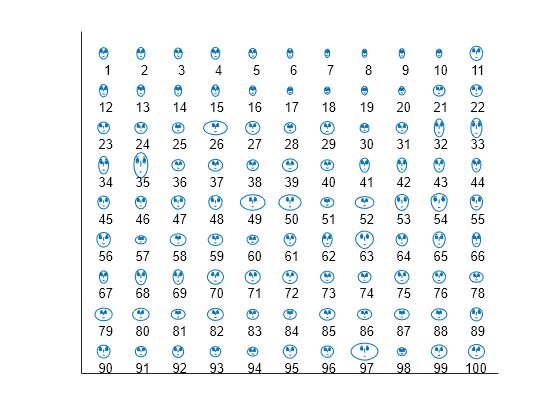

Because the plot does not display the MPG variable, which contained missing values, the plot includes some of the observations omitted from the previous plot.

Specify the layout of the glyphs in a glyph plot. You can specify the grid in which to plot the glyphs or the location of the glyph centers.

Load the carsmall data set, which contains measurements for 100 cars. Combine the Acceleration, Displacement, Horsepower, MPG, and Weight variables into a table. Display the values for the first 12 cars.

load carsmall
Tbl = table(Acceleration,Displacement,Horsepower,MPG,Weight);
head(Tbl,12)

    Acceleration    Displacement    Horsepower    MPG    Weight
    ____________    ____________    __________    ___    ______

          12            307            130         18     3504 
        11.5            350            165         15     3693 
          11            318            150         18     3436 
          12            304            150         16     3433 
        10.5            302            140         17     3449 
          10            429            198         15     4341 
           9            454            220         14     4354 
         8.5            440            215         14     4312 
          10            455            225         14     4425 
         8.5            390            190         15     3850 
        17.5            133            115        NaN     3090 
        11.5            350            165        NaN     4142 

Create a star plot using the car measurements in Tbl. Arrange the stars into an 8-by-12 grid.

glyphplot(Tbl{:,:},Grid=[8 12])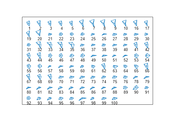

Because the grid is 8-by-12, the plot can display at most 96 observations. In this case, the plot contains all observations in Tbl that do not have missing values. By default, glyphplot labels each glyph with the index of the observation in Tbl.

Display the stars in a 2-by-2 grid. Use the Page name-value argument to specify the set of stars to display. In this case, display the first two sets of stars.

figure
tiledlayout(1,2)
nexttile
glyphplot(Tbl{:,:},Grid=[2 2])
title("First Set of Stars")
nexttile
glyphplot(Tbl{:,:},Grid=[2 2],Page=2)
title("Second Set of Stars")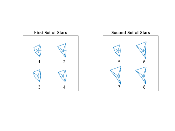

You can also display multiple pages in succession by specifying Page as a numeric vector or "all". After the call to glyphplot, press Enter to display the next page of glyphs.

Alternatively, display all sets of stars in one plot with a scroll bar.

glyphplot(Tbl{:,:},Grid=[2 2],Page="scroll")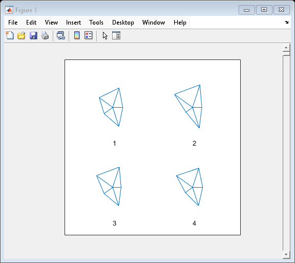

Instead of creating a grid of glyphs, you can specify the location of the glyph centers.

Plot the stars for the first four cars. Standardize the data set before passing it to glyphplot. Otherwise, the function standardizes only the four observations, instead of the entire data set, before plotting. Specify the star center locations as a matrix, with row i corresponding to the x- and y-axis values, respectively, of star center i. Specify the maximum star radius as 0.5. To better compare the stars, add grid lines to the plot.

figure
X = normalize(Tbl{:,:},"range",[0.1 0.9]);
glyphplot(X(1:4,:),Centers=[1 2; 2 2; 1 1; 2 1],Radius=0.5, ...
    Standardize="off")
grid on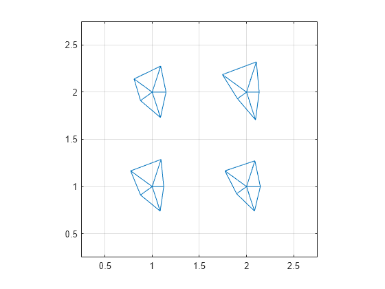

When you specify the location of the glyph centers, the glyph plot does not include observation labels.

Adjust the appearance of a glyph plot by setting some plot properties in the call to glyphplot, and by modifying the appearance of the plot after creating it.

Load the fisheriris data set, which contains four measurements (sepal length, sepal width, petal length, and petal width) from three species of iris flowers.

load fisheriris

The matrix meas contains all four measurements for 150 flowers. The cell array species contains the species name for each of the 150 flowers.

Create a new variable named label that contains the index and species name for each flower.

index = (1:150)';
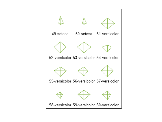
label = index + "-" + species;

Create a star plot using the iris measurements in meas, and label each star using the label variable. Specify the color of the stars as light green. When you specify line properties (such as Color) in the call to glyphplot, the function sets the property values for all the glyphs in the plot. For simplicity, display flowers 49–60 in a 4-by-3 grid.

To modify the appearance of the plot after creating it, return an array of Line and Text objects s.

lightGreen = [0.4660 0.6740 0.1880];

s = glyphplot(meas,ObsLabels=label, ...
    Color=lightGreen, ...
    Grid=[4 3],Page=5);

For the star corresponding to flower 51, modify the color of the star perimeter, the color of the star spokes, and the font of the star label.

purple = [0.4940 0.1840 0.5560];
lightBlue = [0.3010 0.7450 0.9330];

s(3,1).Color = purple;
s(3,2).Color = lightBlue;
s(3,3).FontWeight = "bold";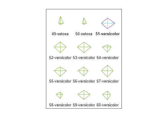

The star corresponding to flower 51 has a purple outline, light blue spokes, and a bold label.

Recreate the previous plot using a face plot instead of a star plot. Return and modify an array of Line and Text objects f.

figure
f = glyphplot(meas,Glyph="face",ObsLabels=label, ...
    Color=lightGreen, ...
    Grid=[4 3],Page=5);
f(3,1).Color = purple;
f(3,2).Color = lightBlue;
f(3,3).FontWeight = "bold";

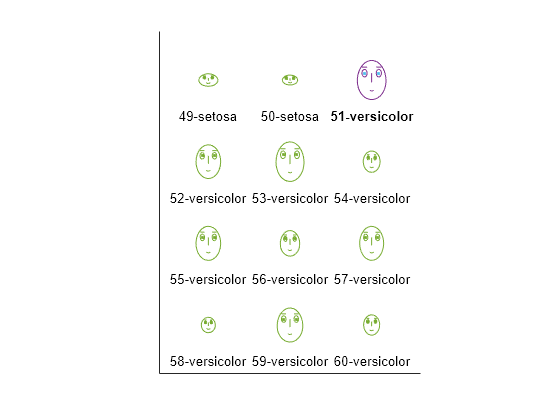
The face corresponding to flower 51 has a purple face, light blue eyes, and a bold label.