Main Content

mvncdf

Multivariate normal cumulative distribution function

Description

p = mvncdf(X) returns the cumulative distribution function (cdf) of the multivariate normal distribution with zero mean and identity covariance matrix, evaluated at each row of X. For more information, see Multivariate Normal Distribution.

example

p = mvncdf(X,mu,Sigma) returns the cdf of the multivariate normal distribution with mean mu and covariance Sigma, evaluated at each row of X.

Specify [] for mu to use its default value of zero when you want to specify only Sigma.

example

p = mvncdf(xl,xu,mu,Sigma) returns the multivariate normal cdf evaluated over the multidimensional rectangle with lower and upper limits defined by xl and xu, respectively.

example

p = mvncdf(___,options) specifies control parameters for the numerical integration used to compute p, using any of the input argument combinations in the previous syntaxes. Create the options argument using the statset function with any combination of the parameters 'TolFun', 'MaxFunEvals', and 'Display'.

example

[p,err] = mvncdf(___) additionally returns an estimate of the error in p. For more information, see Algorithms.

example

Examples

collapse all

Evaluate the cdf of a standard four-dimensional multivariate normal distribution at points with increasing coordinates in every dimension.

Create a matrix X of five four-dimensional points with increasing coordinates.

firstDim = (-2:2)';
X = repmat(firstDim,1,4)
X = 5×4

    -2    -2    -2    -2
    -1    -1    -1    -1
     0     0     0     0
     1     1     1     1
     2     2     2     2

Evaluate the cdf at the points in X.

p = mvncdf(X)
p = 5×1

    0.0000
    0.0006
    0.0625
    0.5011
    0.9121

The cdf values increase because the coordinates of the points are increasing in every dimension.

Compute and plot the cdf of a bivariate normal distribution.

Define the mean vector mu and the covariance matrix Sigma.

mu = [1 -1];
Sigma = [.9 .4; .4 .3];

Create a grid of 625 evenly spaced points in two-dimensional space.

[X1,X2] = meshgrid(linspace(-1,3,25)',linspace(-3,1,25)');
X = [X1(:) X2(:)];

Evaluate the cdf of the normal distribution at the grid points.

p = mvncdf(X,mu,Sigma);

Plot the cdf values.

Z = reshape(p,25,25);
surf(X1,X2,Z)

Figure contains an axes object. The axes object contains an object of type surface.

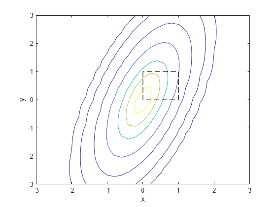
Compute the probability over the unit square of a bivariate normal distribution, and create a contour plot of the results.

Define the bivariate normal distribution parameters mu and Sigma.

mu = [0 0];
Sigma = [0.25 0.3; 0.3 1];

Compute the probability over the unit square.

p = mvncdf([0 0],[1 1],mu,Sigma)
p = 
0.2097

To visualize the result, first create a grid of evenly spaced points in two-dimensional space.

x1 = -3:.2:3;
x2 = -3:.2:3;
[X1,X2] = meshgrid(x1,x2);
X = [X1(:) X2(:)];

Then, evaluate the pdf of the normal distribution at the grid points.

y = mvnpdf(X,mu,Sigma);
y = reshape(y,length(x2),length(x1));

Finally, create a contour plot of the multivariate normal distribution that includes the unit square.

contour(x1,x2,y,[0.0001 0.001 0.01 0.05 0.15 0.25 0.35])
xlabel('x')
ylabel('y')
line([0 0 1 1 0],[1 0 0 1 1],'Linestyle','--','Color','k')

Figure contains an axes object. The axes object with xlabel x, ylabel y contains 2 objects of type contour, line.

Computing a multivariate cumulative probability requires significantly more work than computing a univariate probability. By default, the mvncdf function computes values to less than full machine precision, and returns an estimate of the error as an optional second output. View the error estimate in this case.

[p,err] = mvncdf([0 0],[1 1],mu,Sigma)
p = 
0.2097
err = 
1.0000e-08

Evaluate the cdf of a multivariate normal distribution at random points, and display the error estimates associated with the cdf calculation.

Generate four random points from a five-dimensional multivariate normal distribution with mean vector mu and covariance matrix Sigma.

mu = [0.5 -0.3 0.2 0.1 -0.4];
Sigma = 0.5*eye(5);
rng('default')  % For reproducibility
X = mvnrnd(mu,Sigma,4);

Find the cdf values p at the points in X and the associated error estimates err. Display a summary of the numerical calculations.

[p,err] = mvncdf(X,mu,Sigma,statset('Display','final'))
Successfully satisfied error tolerance of 0.0001 in 8650 function evaluations.
p = 4×1

    0.1520
    0.0407
    0.0002
    0.1970

err = 4×1
10-16 ×

    0.5949
    0.1487
         0
    0.1983

Input Arguments

collapse all

Evaluation points, specified as an n-by-d numeric matrix, where n is a positive scalar integer and d is the dimension of a single multivariate normal distribution. The rows of X correspond to observations (or points), and the columns correspond to variables (or coordinates).

Data Types: single | double

Mean vector of a multivariate normal distribution, specified as a 1-by-d numeric vector or a numeric scalar, where d is the dimension of the multivariate normal distribution. If mu is a scalar, then mvncdf replicates the scalar to match the size of X.

Data Types: single | double

Covariance matrix of a multivariate normal distribution, specified as a d-by-d symmetric, positive definite matrix, where d is the dimension of the multivariate normal distribution. If the covariance matrix is diagonal, containing variances along the diagonal and zero covariances off it, then you can also specify Sigma as a 1-by-d vector containing just the diagonal entries.

Data Types: single | double

Rectangle lower limit, specified as a 1-by-d numeric vector.

Data Types: single | double

Rectangle upper limit, specified as a 1-by-d numeric vector.

Data Types: single | double

Numerical integration options, specified as a structure. Create the options argument by calling the statset function with any combination of the following parameters:

  • 'TolFun' — Maximum absolute error tolerance. The default value is 1e-8 when d < 4, and 1e-4 when d ≥ 4.

  • 'MaxFunEvals' — Maximum number of integrand evaluations allowed when d ≥ 4. The default value is 1e7. The function ignores 'MaxFunEvals' when d < 4.

  • 'Display' — Level of display output. The choices are 'off' (the default), 'iter', and 'final'. The function ignores 'Display' when d < 4.

Example: statset('TolFun',1e-7,'Display','final')

Data Types: struct

Output Arguments

collapse all

cdf values, returned as either an n-by-1 numeric vector, where n is the number of rows in X, or a numeric scalar representing the probability over the rectangular region specified by xl and xu.

Absolute error tolerance, returned as a positive numeric scalar. For bivariate and trivariate distributions, the default absolute error tolerance is 1e-8. For four or more dimensions, the default absolute error tolerance is 1e-4. For more information, see Algorithms.

More About

collapse all

Multivariate Normal Distribution

The multivariate normal distribution is a generalization of the univariate normal distribution to two or more variables. It has two parameters, a mean vector μ and a covariance matrix Σ, that are analogous to the mean and variance parameters of a univariate normal distribution. The diagonal elements of Σ contain the variances for each variable, and the off-diagonal elements of Σ contain the covariances between variables.

The probability density function (pdf) of the d-dimensional multivariate normal distribution is

y = f(x,μ,Σ) = 1|Σ|(2π)dexp(12(x-μΣ-1(x-μ)')

where x and μ are 1-by-d vectors and Σ is a d-by-d symmetric, positive definite matrix. Only mvnrnd allows positive semi-definite Σ matrices, which can be singular. The pdf cannot have the same form when Σ is singular.

The multivariate normal cumulative distribution function (cdf) evaluated at x is the probability that a random vector v, distributed as multivariate normal, lies within the semi-infinite rectangle with upper limits defined by x:

Pr{v(1)x(1),v(2)x(2),...,v(d)x(d)}.

Although the multivariate normal cdf does not have a closed form, mvncdf can compute cdf values numerically.

Tips

  • In the one-dimensional case, Sigma is the variance, not the standard deviation. For example, mvncdf(1,0,4) is the same as normcdf(1,0,2), where 4 is the variance and 2 is the standard deviation.

Algorithms

For bivariate and trivariate distributions, mvncdf uses adaptive quadrature on a transformation of the t density, based on methods developed by Drezner and Wesolowsky [1] [2] and by Genz [3]. For four or more dimensions, mvncdf uses a quasi-Monte Carlo integration algorithm based on methods developed by Genz and Bretz [4] [5].

References

[1] Drezner, Z. “Computation of the Trivariate Normal Integral.” Mathematics of Computation. Vol. 63, 1994, pp. 289–294.

[2] Drezner, Z., and G. O. Wesolowsky. “On the Computation of the Bivariate Normal Integral.” Journal of Statistical Computation and Simulation. Vol. 35, 1989, pp. 101–107.

[3] Genz, A. “Numerical Computation of Rectangular Bivariate and Trivariate Normal and t Probabilities.” Statistics and Computing. Vol. 14, No. 3, 2004, pp. 251–260.

[4] Genz, A., and F. Bretz. “Numerical Computation of Multivariate t Probabilities with Application to Power Calculation of Multiple Contrasts.” Journal of Statistical Computation and Simulation. Vol. 63, 1999, pp. 361–378.

[5] Genz, A., and F. Bretz. “Comparison of Methods for the Computation of Multivariate t Probabilities.” Journal of Computational and Graphical Statistics. Vol. 11, No. 4, 2002, pp. 950–971.

[6] Kotz, S., N. Balakrishnan, and N. L. Johnson. Continuous Multivariate Distributions: Volume 1: Models and Applications. 2nd ed. New York: John Wiley & Sons, Inc., 2000.

Extended Capabilities

Version History

Introduced in R2006a