Random Subspace Classification

Open Live Script

This example shows how to use a random subspace ensemble to increase the accuracy of classification. It also shows how to use cross validation to determine good parameters for both the weak learner template and the ensemble.

Load the data

Load the ionosphere data. This data has 351 binary responses to 34 predictors.

load ionosphere;
[N,D] = size(X)

N = 
351

D = 
34

resp = unique(Y)

resp = 2x1 cell
    {'b'}
    {'g'}

Choose the number of nearest neighbors

Find a good choice for k, the number of nearest neighbors in the classifier, by cross validation. Choose the number of neighbors approximately evenly spaced on a logarithmic scale.

rng(8000,'twister') % for reproducibility
K = round(logspace(0,log10(N),10)); % number of neighbors 
cvloss = zeros(numel(K),1);
for k=1:numel(K)
    knn = fitcknn(X,Y,...
        'NumNeighbors',K(k),'CrossVal','On');
    cvloss(k) = kfoldLoss(knn);
end
figure; % Plot the accuracy versus k
semilogx(K,cvloss);
xlabel('Number of nearest neighbors');
ylabel('10 fold classification error');
title('KNN classification');

Figure contains an axes object. The axes object with title KNN classification, xlabel Number of nearest neighbors, ylabel 10 fold classification error contains an object of type line.

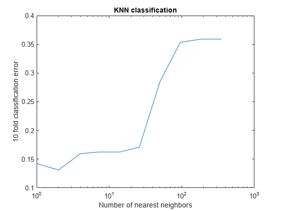
The lowest cross-validation error occurs for k = 2.

Create the ensembles

Create ensembles for 2-nearest neighbor classification with various numbers of dimensions, and examine the cross-validated loss of the resulting ensembles.

This step takes a long time. To keep track of the progress, print a message as each dimension finishes.

NPredToSample = round(linspace(1,D,10)); % linear spacing of dimensions
cvloss = zeros(numel(NPredToSample),1);
learner = templateKNN('NumNeighbors',2);
for npred=1:numel(NPredToSample)
   subspace = fitcensemble(X,Y,'Method','Subspace','Learners',learner, ...
       'NPredToSample',NPredToSample(npred),'CrossVal','On');
   cvloss(npred) = kfoldLoss(subspace);
   fprintf('Random Subspace %i done.\n',npred);
end

Random Subspace 1 done.
Random Subspace 2 done.
Random Subspace 3 done.
Random Subspace 4 done.
Random Subspace 5 done.
Random Subspace 6 done.
Random Subspace 7 done.
Random Subspace 8 done.
Random Subspace 9 done.
Random Subspace 10 done.

figure; % plot the accuracy versus dimension
plot(NPredToSample,cvloss);
xlabel('Number of predictors selected at random');
ylabel('10 fold classification error');
title('KNN classification with Random Subspace');

Figure contains an axes object. The axes object with title KNN classification with Random Subspace, xlabel Number of predictors selected at random, ylabel 10 fold classification error contains an object of type line.

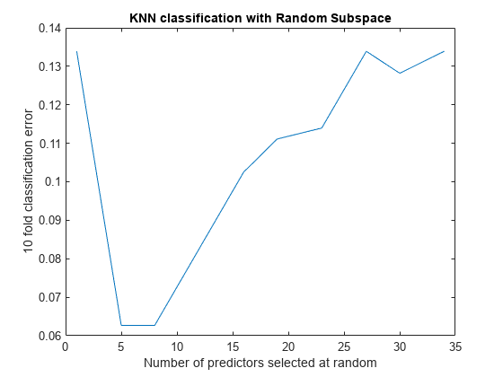
The ensembles that use five and eight predictors per learner have the lowest cross-validated error. The error rate for these ensembles is about 0.06, while the other ensembles have cross-validated error rates that are approximately 0.1 or more.

Find a good ensemble size

Find the smallest number of learners in the ensemble that still give good classification.

ens = fitcensemble(X,Y,'Method','Subspace','Learners',learner, ...
       'NPredToSample',5,'CrossVal','on');
figure; % Plot the accuracy versus number in ensemble
plot(kfoldLoss(ens,'Mode','Cumulative'))
xlabel('Number of learners in ensemble');
ylabel('10 fold classification error');
title('KNN classification with Random Subspace');

Figure contains an axes object. The axes object with title KNN classification with Random Subspace, xlabel Number of learners in ensemble, ylabel 10 fold classification error contains an object of type line.

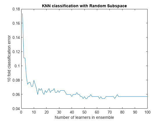
There seems to be no advantage in an ensemble with more than 50 or so learners. It is possible that 25 learners gives good predictions.

Create a final ensemble

Construct a final ensemble with 50 learners. Compact the ensemble and see if the compacted version saves an appreciable amount of memory.

ens = fitcensemble(X,Y,'Method','Subspace','NumLearningCycles',50,...
    'Learners',learner,'NPredToSample',5);
cens = compact(ens);
s1 = whos('ens');
s2 = whos('cens');
[s1.bytes s2.bytes] % si.bytes = size in bytes

ans = 1×2

     1760497     1529060

The compact ensemble is about 10% smaller than the full ensemble. Both give the same predictions.