Train Regression Trees Using Regression Learner App
This example shows how to create and compare various regression trees using the Regression Learner app, and export trained models to the workspace to make predictions for new data.
You can train regression trees to predict responses to given input data. To predict the response of a regression tree, follow the tree from the root (beginning) node down to a leaf node. At each node, decide which branch to follow using the rule associated to that node. Continue until you arrive at a leaf node. The predicted response is the value associated to that leaf node.
Statistics and Machine Learning Toolbox™ trees are binary. Each step in a prediction involves checking the value of one predictor variable. For example, here is a simple regression tree:

This tree predicts the response based on two predictors, x1 and
x2. To predict, start at the top node. At each node, check the
values of the predictors to decide which branch to follow. When the branches reach a
leaf node, the response is set to the value corresponding to that node.
This example uses the carbig data set. This data set contains
characteristics of different car models produced from 1970 through 1982,
including:
Acceleration
Number of cylinders
Engine displacement
Engine power (Horsepower)
Model year
Weight
Country of origin
Miles per gallon (MPG)
Train regression trees to predict the fuel economy in miles per gallon of a car model, given the other variables as inputs.
In MATLAB®, load the
carbigdata set and create a table containing the different variables:load carbig cartable = table(Acceleration,Cylinders,Displacement, ... Horsepower,Model_Year,Weight,Origin,MPG);
On the Apps tab, in the Machine Learning and Deep Learning group, click Regression Learner.
On the Learn tab, in the File section, select New Session > From Workspace.
Under Data Set Variable in the New Session from Workspace dialog box, select
cartablefrom the list of tables and matrices in your workspace.Observe that the app has preselected response and predictor variables.
MPGis chosen as the response, and all the other variables as predictors. For this example, do not change the selections.
To accept the default validation scheme and continue, click Start Session. The default validation option is cross-validation, to protect against overfitting.
Regression Learner creates a plot of the response with the record number on the x-axis.
Use the response plot to investigate which variables are useful for predicting the response. To visualize the relation between different predictors and the response, select different variables in the X list under X-axis to the right of the plot.
Observe which variables are correlated most clearly with the response.
Displacement,Horsepower, andWeightall have a clearly visible impact on the response and all show a negative association with the response.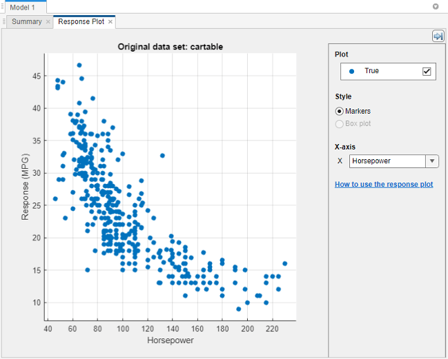
Select the variable
Originunder X-axis. A box plot is automatically displayed. A box plot shows the typical values of the response and any possible outliers. The box plot is useful when plotting markers results in many points overlapping. To show a box plot when the variable on the x-axis has few unique values, under Style, select Box plot.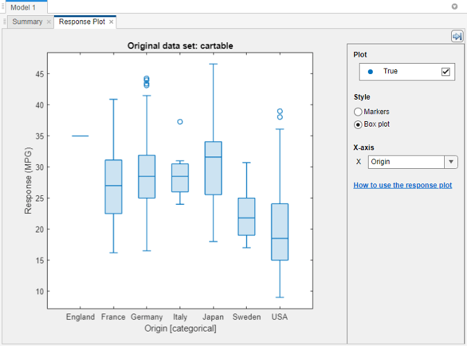
Train a selection of regression trees. The Models pane already contains a fine tree model. Add medium and coarse tree models to the list of draft models. On the Learn tab, in the Models section, click the arrow to open the gallery. In the Regression Trees group, click Medium Tree. The app creates a draft medium tree in the Models pane. Reopen the model gallery and click Coarse Tree in the Regression Trees group. The app creates a draft coarse tree in the Models pane.
In the Train section, click Train All and select Train All. The app trains the three tree models and plots both the true training response and the predicted response for each model.
Note
If you have Parallel Computing Toolbox™, then the Use Parallel button is selected by default. After you click Train All and select Train All or Train Selected, the app opens a parallel pool of workers. During this time, you cannot interact with the software. After the pool opens, you can continue to interact with the app while models train in parallel.
If you do not have Parallel Computing Toolbox, then the Use Background Training check box in the Train All menu is selected by default. After you select an option to train models, the app opens a background pool. After the pool opens, you can continue to interact with the app while models train in the background.

Note
Validation introduces some randomness into the results. Your model validation results can vary from the results shown in this example.
In the Models pane, check the RMSE (Validation) (validation root mean squared error) of the models. The best score is highlighted in a box.
The Fine Tree and the Medium Tree have similar RMSEs, while the Coarse Tree is less accurate.
Choose a model in the Models pane to view the results of that model. For example, select the Medium Tree model (model 2). In the Response Plot tab, under X-axis, select
Horsepowerand examine the response plot. Both the true and predicted responses are now plotted. Show the prediction errors, drawn as vertical lines between the predicted and true responses, by selecting the Errors check box.See more details on the currently selected model in the model's Summary tab. To open this tab, right-click the model and select Summary. Check and compare additional model characteristics, such as R2 (coefficient of determination), MAE (mean absolute error), and prediction speed. To learn more, see View Model Metrics in Summary Tab and Models Pane. In the Summary tab, you also can find details on the currently selected model type, such as the hyperparameters used for training the model.
Plot the predicted response versus true response. On the Learn tab, in the Plots and Results section, click the arrow to open the gallery, and then click Predicted vs. Actual (Validation) in the Validation Results group. Use this plot to understand how well the regression model makes predictions for different response values.
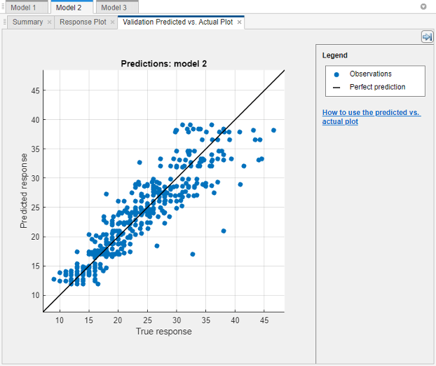
A perfect regression model has predicted response equal to true response, so all the points lie on a diagonal line. The vertical distance from the line to any point is the error of the prediction for that point. A good model has small errors, so the predictions are scattered near the line. Usually a good model has points scattered roughly symmetrically around the diagonal line. If you can see any clear patterns in the plot, it is likely that you can improve your model.
Select the other models in the Models pane, open the predicted versus actual plot for each of the models, and then compare the results. Rearrange the layout of the plots to better compare the plots. Click the Document Actions button located to the far right of the model plot tabs. Select the
Tile Alloption and specify a 1-by-3 layout. Click the Hide plot options button at the top right of the plots to make more
room for the plots.
at the top right of the plots to make more
room for the plots.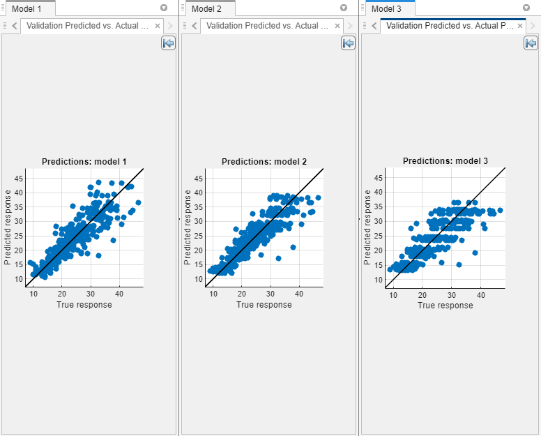
To return to the original layout, you can click the Layout button in the Plots and Results section and select Single model (Default).
In the Models gallery, select All Trees in the Regression Trees group. To try to improve the tree models, include different features in the models. See if you can improve the model by removing features with low predictive power.
On the Learn tab, in the Options section, click Feature Selection.
In the Default Feature Selection tab, you can select different feature ranking algorithms to determine the most important features. After you select a feature ranking algorithm, the app displays a plot of the sorted feature importance scores, where larger scores (including
Infs) indicate greater feature importance. The table shows the ranked features and their scores.In this example, both the MRMR and F Test feature ranking algorithms rank the acceleration and country of origin predictors the lowest. The app disables the RReliefF option because the predictors include a mix of numeric and categorical variables.
Under Feature Ranking Algorithm, click F Test. Under Feature Selection, use the default option of selecting the highest ranked features to avoid bias in the validation metrics. Specify to keep 4 of the 7 features for model training.

Click Save and Apply. The app applies the feature selection changes to the current draft model and any new models created using the Models gallery.
Train the tree models using the reduced set of features. On the Learn tab, in the Train section, click Train All and select Train All or Train Selected.
Observe the new models in the Models pane. These models are the same regression trees as before, but trained using only 4 of 7 predictors. The app displays how many predictors are used. To check which predictors are used, click a model in the Models pane, and note the check boxes in the expanded Feature Selection section of the model Summary tab.
Note
If you use a cross-validation scheme and choose to perform feature selection using the Select highest ranked features option, then for each training fold, the app performs feature selection before training a model. Different folds can select different predictors as the highest ranked features. The table on the Default Feature Selection tab shows the list of predictors used by the full model, trained on the training and validation data.
The models with the three features removed do not perform as well as the models using all predictors. In general, if data collection is expensive or difficult, you might prefer a model that performs satisfactorily without some predictors.
Train the three regression tree presets using only
Horsepoweras a predictor. In the Models gallery, select All Trees in the Regression Trees group. In the model Summary tab, expand the Feature Selection section. Choose the Select individual features option, and clear the check boxes for all features exceptHorsepower. On the Learn tab, in the Train section, click Train All and select Train Selected.Using only the engine power as a predictor results in models with lower accuracy. However, the models perform well given that they are using only a single predictor. With this simple one-dimensional predictor space, the coarse tree now performs as well as the medium and fine trees.
Select the best model in the Models pane and view the residuals plot. On the Learn tab, in the Plots and Results section, click the arrow to open the gallery, and then click Residuals (Validation) in the Validation Results group. The residuals plot displays the difference between the predicted and true responses. To display the residuals as a line graph, in the Style section, choose Lines.
Under X-axis, select the variable to plot on the x-axis. Choose the true response, predicted response, record number, or one of the predictors.
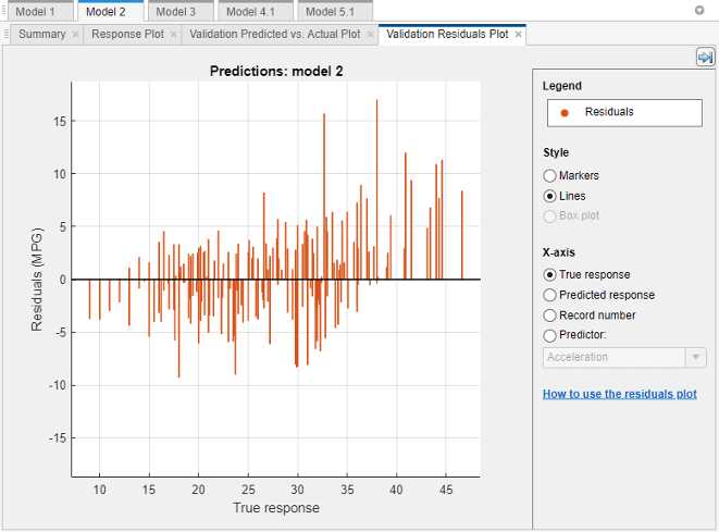
Usually a good model has residuals scattered roughly symmetrically around 0. If you can see any clear patterns in the residuals, it is likely that you can improve your model.
To learn about model hyperparameter settings, choose the best model in the Models pane and expand the Model Hyperparameters section in the model Summary tab. Compare the coarse, medium, and fine tree models, and note the differences in the model hyperparameters. In particular, the Minimum leaf size setting is 36 for coarse trees, 12 for medium trees, and 4 for fine trees. This setting controls the size of the tree leaves, and through that the size and depth of the regression tree.
To try to improve the best model (the medium tree trained using all predictors), change the Minimum leaf size setting. First, click the model in the Models pane. Right-click the model and select Duplicate. In the Summary tab, change the Minimum leaf size value to 8. Then, in the Train section of the Learn tab, click Train All and select Train Selected.
To learn more about regression tree settings, see Regression Trees.
You can export a full or compact version of the selected model to the workspace. In the Export section of the Learn tab, click Export Model and select Export Model to Workspace. To exclude the training data and export a compact model, clear the check box in the Export Regression Model dialog box. You can still use the compact model for making predictions on new data. In the dialog box, click OK to accept the default variable name
trainedModel.The Command Window displays information about the results.
Use the exported model to make predictions on new data. For example, to make predictions for the
cartabledata in your workspace, enter:The outputyfit = trainedModel.predictFcn(cartable)
yfitcontains the predicted response for each data point.If you want to automate training the same model with new data or learn how to programmatically train regression models, you can generate code from the app. To generate code for the best trained model, on the Learn tab, in the Export section, click Generate Function.
The app generates code from your model and displays the file in the MATLAB Editor. To learn more, see Generate MATLAB Code to Train Model with New Data.
Tip
Use the same workflow as in this example to evaluate and compare the other regression model types you can train in Regression Learner.
Train all the nonoptimizable regression model presets available:
On the Learn tab, in the Models section, click the arrow to open the gallery of regression models.
In the Get Started group, click All.
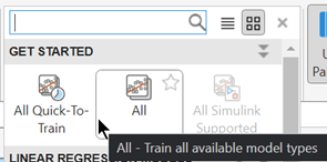
In the Train section, click Train All and select Train All.
To learn about other regression model types, see Train Regression Models in Regression Learner App.
See Also
Topics
- Train Regression Models in Regression Learner App
- Select Data for Regression or Open Saved App Session
- Choose Regression Model Options
- Feature Selection and Feature Transformation Using Regression Learner App
- Visualize and Assess Model Performance in Regression Learner
- Export Regression Model to Predict New Data