主要内容

umap

Uniform Manifold Approximation and Projection (UMAP) for dimension reduction

Since R2026a

Description

Y = umap(X) returns a matrix of lower-dimensional embeddings of the high-dimensional rows of X. To calculate the embeddings, the function uses the Neg-t-SNE version of the Uniform Manifold Approximation and Projection (UMAP) algorithm for dimension reduction. For more information, see Algorithms.

example

Y = umap(X,Name=Value) modifies the embeddings using options specified by one or more name-value arguments. For example, you can specify the distance metric or the initialization method for the low-dimensional embedding.

example

[Y,NeighborIndicesResult] = umap(___) also returns the NumNeighbors nearest neighbor row indices for each row of X that does not contain any NaN values. Use this syntax with any of the input arguments in the previous syntaxes.

Examples

collapse all

View the 2-D and 3-D embeddings of the human activity data set using the umap function.

Load the data set.

load humanactivity

The data set contains 24,075 observations of 60 predictors, and an activity class label for each observation. For more details on the data set, enter Description at the command line.

Associate the activities with the labels in actid.

activities = ["Sitting";"Standing";"Walking";"Running";"Dancing"];
activity = activities(actid);

Because UMAP is a stochastic algorithm, set the random number seed.

rng(0,"twister") % For reproducibility

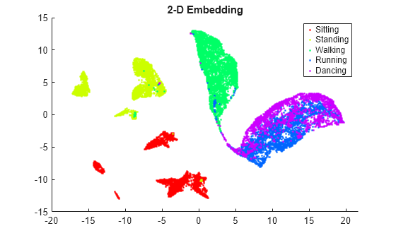
View the 2-D embedding. Assign a color to each activity class using the hsv colormap.

Y2 = umap(feat);   % Default number of embedding dimensions is 2
figure
colormap = hsv(5);
gscatter(Y2(:,1),Y2(:,2),activity,colormap)
title("2-D Embedding")

Figure contains an axes object. The axes object with title 2-D Embedding contains 5 objects of type line. One or more of the lines displays its values using only markers These objects represent Sitting, Standing, Walking, Running, Dancing.

View the 3-D embedding.

Y3= umap(feat,NumDimensions=3);
figure
scatter3(Y3(:,1),Y3(:,2),Y3(:,3),8,colormap(actid,:),"filled")
title("3-D Embedding")
grid on
view([12 60])

Figure contains an axes object. The axes object with title 3-D Embedding contains an object of type scatter.

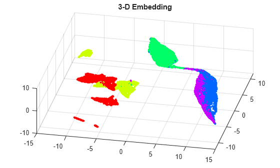
By rotating the 3-D plot, you can see that the activities Running and Dancing are more easily distinguished in 3-D than in 2-D.

Determine the effects of the UMAP embedding density and number of nearest neighbor settings on the two-dimensional embeddings of two data sets: a simulated clustered data set and a human activity data set.

Create Simulated Clustered Data

Create a simulated clustered data set with 1000 observations of 10 predictors. X contains five clusters of 200 observations each. Y contains the cluster identification numbers. The predictor values of each cluster centroid lie within the range [–5,5] and have a standard deviation sigma. The sigma value for each cluster is a random scalar in the range (0,3].

rng(0,"twister"); % For reproducibility
nClusters = 5;
obsPerCluster = 200;
X = [];
Y = [];
xrange = 5;
nPredictors = 10;
sigmaRange = 3;
for c = 1:nClusters
    Y = [Y; c*ones(obsPerCluster,1)];
    sigma = rand*sigmaRange;
    X = [X; randn(obsPerCluster,nPredictors)*sigma + ...
        (randi(2*xrange,[1,nPredictors])-xrange).* ...
        ones(obsPerCluster,nPredictors)];
end

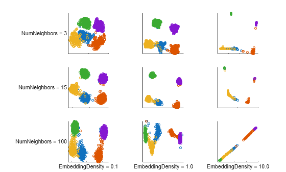
View Two-Dimensional Clustered Data Embeddings

Compute two-dimensional embeddings for X with different parameter settings by using the umap function. Specify 0.1, 1, and 10 for the embedding density values, and 3, 15, and 100 for the number of nearest neighbor values. Because UMAP is a stochastic algorithm, reset the random number seed each time and set Reproducible to true. This setting for Reproducible slows down computations considerably, but is needed in this example to ensure a fair comparison between parameter settings. Display each embedding in a separate plot and assign a different color to each cluster identification number.

density = [0.1 1 10 0.1 1 10 0.1 1 10];
nNeighbors = [3 3 3 15 15 15 100 100 100];

figure
t = tiledlayout(3,3,TileSpacing="compact",Padding="compact");

for i = 1:9
    rng(0,"twister"); % For fair comparison
    E1 = umap(X,EmbeddingDensity=density(i), ...
        NumNeighbors=nNeighbors(i),Reproducible=false);
    ax = nexttile;
    gscatter(E1(:,1),E1(:,2),Y,[],"o",3,"off")
    ax.XTickLabel = [];
    ax.YTickLabel = [];
    if i > 6
        xlabel(sprintf("EmbeddingDensity = %.1f",density(i)),FontSize=8);
    end
    if (mod(i-1,3) == 0)
        ylabel(sprintf("NumNeighbors = %d",nNeighbors(i)), ...
            FontSize=8,Rotation=0); 
    end
    axis square
end

Figure contains 9 axes objects. Axes object 1 with ylabel NumNeighbors = 3 contains 5 objects of type line. One or more of the lines displays its values using only markers Axes object 2 contains 5 objects of type line. One or more of the lines displays its values using only markers Axes object 3 contains 5 objects of type line. One or more of the lines displays its values using only markers Axes object 4 with ylabel NumNeighbors = 15 contains 5 objects of type line. One or more of the lines displays its values using only markers Axes object 5 contains 5 objects of type line. One or more of the lines displays its values using only markers Axes object 6 contains 5 objects of type line. One or more of the lines displays its values using only markers Axes object 7 with xlabel EmbeddingDensity = 0.1, ylabel NumNeighbors = 100 contains 5 objects of type line. One or more of the lines displays its values using only markers Axes object 8 with xlabel EmbeddingDensity = 1.0 contains 5 objects of type line. One or more of the lines displays its values using only markers Axes object 9 with xlabel EmbeddingDensity = 10.0 contains 5 objects of type line. One or more of the lines displays its values using only markers

Load and Preprocess Human Activity Data

Load the human activity data set.

load humanactivity

The data set contains 24,075 observations of 60 predictors, and an activity class label for each observation. For more details on the data set, enter Description at the command line.

The observations are organized by activity class. To better represent a random set of data, shuffle the rows.

n = numel(actid); 
idx = randsample(n,n); 
X2 = feat(idx,:); 
actid = actid(idx);

View Two-Dimensional Human Activity Data Embeddings

Compute two-dimensional embeddings using standardized data and the same set of embedding density values and number of nearest neighbor values as for the simulated clustered data set. Reset the random number seed before computing each embedding, and set Reproducible=true to ensure a fair comparison between parameter settings. Display each embedding in a separate plot, and assign a different color to each activity class.

figure
t = tiledlayout(3,3,TileSpacing="compact",Padding= "compact");

for i = 1:9
    rng(0,"twister"); % For fair comparison
    E2 = umap(X2,Standardize=true,EmbeddingDensity=density(i), ...
        NumNeighbors=nNeighbors(i),Reproducible=true);

    ax = nexttile;
    gscatter(E2(:,1),E2(:,2),actnames(actid)',[],"o",3,"off")
    ax.XTickLabel = [];
    ax.YTickLabel = [];
    if i > 6
        xlabel(sprintf("EmbeddingDensity = %.1f",density(i)),FontSize=8);
    end
    if (mod(i-1,3) == 0)
        ylabel(sprintf("NumNeighbors = %d",nNeighbors(i)), ...
            FontSize=8,Rotation=0); 
    end
    axis square
end

Figure contains 9 axes objects. Axes object 1 with ylabel NumNeighbors = 3 contains 5 objects of type line. One or more of the lines displays its values using only markers Axes object 2 contains 5 objects of type line. One or more of the lines displays its values using only markers Axes object 3 contains 5 objects of type line. One or more of the lines displays its values using only markers Axes object 4 with ylabel NumNeighbors = 15 contains 5 objects of type line. One or more of the lines displays its values using only markers Axes object 5 contains 5 objects of type line. One or more of the lines displays its values using only markers Axes object 6 contains 5 objects of type line. One or more of the lines displays its values using only markers Axes object 7 with xlabel EmbeddingDensity = 0.1, ylabel NumNeighbors = 100 contains 5 objects of type line. One or more of the lines displays its values using only markers Axes object 8 with xlabel EmbeddingDensity = 1.0 contains 5 objects of type line. One or more of the lines displays its values using only markers Axes object 9 with xlabel EmbeddingDensity = 10.0 contains 5 objects of type line. One or more of the lines displays its values using only markers

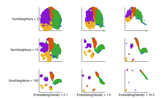
The embeddings of the two data sets show that higher embedding density values result in a tighter clustering of points. For very high values of EmbeddingDensity, the clusters can begin to merge. The effect of the number of nearest neighbors parameter depends on the particular data set and the embedding density value. A higher value of NumNeighbors causes umap to treat more pairs of points as neighbors, and to try bringing them closer together in the embedding space.

For the simulated clustered data set, the tightest, most distinct cluster representation occurs for NumNeighbors = 15. However, when EmbeddingDensity is 10, none of the NumNeighbors values yield an embedding with distinct clusters.

For the human activity data set, the highest NumNeighbors value yields relatively distinct clusters. However, when NumNeighbors is 100 and EmbeddingDensity is 10, most of the observations overlap in the same locations.

Input Arguments

collapse all

Data points, specified as a numeric matrix with m columns, or as a table with m variables. Each row of X contains one m-dimensional point. X must have at least two rows that do not contain a NaN value. umap ignores rows of X that contain at least one NaN value.

Data Types: single | double

Name-Value Arguments

expand all

Specify optional pairs of arguments as Name1=Value1,...,NameN=ValueN, where Name is the argument name and Value is the corresponding value. Name-value arguments must appear after other arguments, but the order of the pairs does not matter.

Example: Y = umap(X,NumDimensions=3) computes a three-dimensional embedding for the data points X.

Algorithm Control

expand all

Size of the Gram matrix in megabytes, specified as a positive scalar or "maximal". This argument is valid only when the Distance name-value argument begins with fast.

If you set CacheSize to "maximal", umap tries to allocate enough memory for an entire intermediate matrix whose size is M-by-M, where M is the number of rows of the input data X. The cache size does not have to be large enough for an entire intermediate matrix, but must be at least large enough to hold an M-by-1 vector. Otherwise, umap uses the standard algorithm for computing Euclidean distances.

If the value of CacheSize is too large or "maximal", umap might try to allocate a Gram matrix that exceeds the available memory. In this case, the software issues an error.

Example: CacheSize="maximal"

Data Types: double | char | string

Distance metric, specified as a character vector, string scalar, or function handle, as described in the following table.

ValueDescription
"euclidean"

Euclidean distance (default)

"seuclidean"Standardized Euclidean distance. Each coordinate difference between the rows in X and the query matrix is scaled by dividing by the corresponding element of the standard deviation computed from S = std(X,"omitnan").
"fasteuclidean"Euclidean distance computed by using an alternative algorithm that saves time when the number of columns in X is at least 10. In some cases, this faster algorithm can reduce accuracy. Algorithms starting with "fast" do not support sparse data. For details, see Algorithms.
"fastseuclidean"Standardized Euclidean distance computed by using an alternative algorithm that saves time when the number of columns in X is at least 10. In some cases, this faster algorithm can reduce accuracy. Algorithms starting with "fast" do not support sparse data. For details, see Algorithms.
"mahalanobis"

Mahalanobis distance, computed using the positive definite covariance matrix cov(X,"omitrows")

"cityblock"

City block distance

"minkowski"

Minkowski distance with exponent 2. This distance is the same as the Euclidean distance.

"chebychev"

Chebychev distance, which is the maximum coordinate difference

"cosine"

One minus the cosine of the included angle between observations (treated as vectors)

"correlation"

One minus the sample linear correlation between observations (treated as sequences of values)

"hamming"

Hamming distance, which is the percentage of coordinates that differ

"jaccard"

One minus the Jaccard coefficient, which is the percentage of nonzero coordinates that differ

"spearman"

One minus the sample Spearman's rank correlation between observations (treated as sequences of values)

@distfun

Custom distance function handle. A distance function has the form

function D2 = distfun(ZI,ZJ)
% calculation of distance
...
where

  • ZI is a 1-by-n vector containing a single observation.

  • ZJ is an m2-by-n matrix containing multiple observations. distfun must accept a matrix ZJ with an arbitrary number of observations.

  • D2 is an m2-by-1 vector of distances, and D2(k) is the distance between observations ZI and ZJ(k,:).

If your data is not sparse, you can generally compute distances more quickly by using a built-in distance metric instead of a function handle.

In all cases, umap uses squared pairwise distances to calculate the Cauchy kernel in the joint distribution of X.

Example: Distance="mahalanobis"

Data Types: char | string | function_handle

Factor for adjusting the density of the embedding structure, specified as a positive scalar. A larger EmbeddingDensity value increases the attraction between similar points, resulting in a more continuous embedding with densely packed regions. A smaller EmbeddingDensity value increases the repulsion, leading to a more discrete embedding structure where the points are more widely spread apart.

This argument corresponds to the Z¯ parameter in the Neg-t-SNE algorithm of Damrich et al. [4]. The default value (1) corresponds approximately to the behavior of the original UMAP algorithm of McInnes et al. [6].

Example: EmbeddingDensity=10

Data Types: single | double

Initialization method for the low-dimensional embedding, specified as "pca" or "random". The initial embedding is an n-by-NumDimensions matrix, where n is the number of rows of X that do not contain any NaN values.

  • "pca"— Use principal component analysis (PCA) to initialize the embedding. Before embedding the high-dimensional data, umap first reduces the dimensionality of the data to NumDimensions PCA components by using the pca function. Compared to using random initial positions, this method is generally better at preserving the global structure of the high-dimensional data.

  • "random"— Initialize the embedding using randomly assigned positions.

Example: Initialization="random"

Data Types: char | string

Dimension of the output Y, specified as a positive integer. The default value of NumDimensions is min(2,n), where n is the number of columns in X.

Example: NumDimensions=3

Data Types: single | double

Number of nearest neighbors, specified as a positive integer. A higher value of NumNeighbors causes umap to treat more pairs of points as neighbors, and to try to bring them closer together in the embedding space.

If you specify NeighborIndices, then the default value of NumNeighbors is n, where n is the number of columns in NeighborIndices. If you specify both NeighborIndices and NumNeighbors, then NumNeighbors must equal n.

Example: NumNeighbors=10

Data Types: single | double

Precomputed nearest neighbor indices, specified as a matrix of positive integers. Setting this name-value argument can improve performance by preventing redundant computations. Each row of NeighborIndices contains the indices of the nearest neighbors for the corresponding observation (row) in X (after the function removes any rows in X that contain at least one NaN value). If you specify NumNeighbors, then NeighborIndices must contain NumNeighbors columns.

Data Types: single | double

Flag to enforce reproducibility, specified as "on" or "off", or as a logical 0 (false) or 1 (true). To reproduce the embeddings over repeated runs, specify Reproducible as true and set the seed of the random number generator using rng.

Note

Setting Reproducible to true can cause slower embedding computation times.

Example: Reproducible=true

Data Types: single | double | logical

Flag to normalize the input data, specified as "on" or "off", or as a logical 0 (false) or 1 (true). When the value is true, umap centers and scales each column of X by first subtracting its mean, then dividing by its standard deviation.

When features in X are on different scales, set Standardize to true. The learning process is based on nearest neighbors, so features with large scales might override the contribution of features with small scales.

Example: Standardize=true

Data Types: single | double | logical

Optimization Control

expand all

Number of optimization epochs, specified as a positive integer. A smaller NumEpochs value speeds up computation time, but can lead to a poorly optimized embedding.

Example: NumEpochs=100

Data Types: single | double

Learning rate for the optimization process, specified as a positive scalar.

When LearnRate is too small, umap can converge to a poor local minimum. When LearnRate is too large, the algorithm might not achieve the best possible optimization for the specified value of NumEpochs.

Example: LearnRate=3

Data Types: single | double

Output Arguments

collapse all

Embedded points, returned as an n-by-NumDimensions matrix. Each row represents one embedded point. n is the number of rows of X that do not contain any NaN values.

Nearest neighbors for the data points in X, returned as an n-by-NumNeighbors matrix of row indices, where n is the number of rows of X that do not contain any NaN values.

Algorithms

collapse all

The UMAP algorithm creates a set of embedded points in a low-dimensional space whose relative similarities mimic those of the original high-dimensional points. The embedded points reflect the clustering in the original data. Unlike PCA, which uses a well-quantified linear algorithm, UMAP provides a nonlinear representation of high-dimensional data. This representation can have an arbitrary rotation or mirroring. However, UMAP can capture high-dimensional topological structures in the data that cannot be represented by principal components.

Because the stochastic nature of the UMAP algorithm makes the embedding sensitive to parameters such as the number of nearest neighbors, embedding density, learning rate, number of optimization epochs, and initialization, no "true" embedding solution exists for any particular data set (see UMAP Settings). The default values of these and other parameters are only suggested starting points. A best practice is to run the umap function multiple times using different parameter settings and compare the embeddings to those generated by other algorithms, such as tsne. In general, consider using umap and tsne only as a starting point for further experiments and hypotheses regarding the data.

The umap function uses the Neg-t-SNE version of UMAP developed by Damrich et al. [4]. The Neg-t-SNE algorithm primarily differs from the original UMAP algorithm of McInnes et al. [6] by using a loss function that is less vulnerable to numerical instability, and by incorporating a normalization parameter Z¯ (see EmbeddingDensity) that controls whether the output embedding is more similar to t-SNE or the original UMAP. During optimization of the embedding, the algorithm attempts to pull together pairs of positive samples, which are close together in the high-dimensional space, and push apart negative samples, which are not close together in the high-dimensional space. For each positive pair, umap samples a fixed number of negative samples (m = 5). As a result, the embedding computation times for UMAP are typically much faster than those for t-SNE, making UMAP more suitable for large data sets and for investigating the effects of different parameter settings on the embedding.

References

[1] Albanie, Samuel. Euclidean Distance Matrix Trick. June, 2019. Available at https://samuelalbanie.com/files/Euclidean_distance_trick.pdf.

[2] Böhm, J. N. "Attraction-Repulsion Spectrum in Neighbor Embeddings." Journal of Machine Learning Research , no. 23 (2022): 4118–4149.

[3] Damrich, Sebastian, and Fred A. Hamprecht. "On UMAP's True Loss Function." Neural Information Processing Systems (2021).

[4] Damrich, Sebastian, et al. "From t-SNE to UMAP with Contrastive Learning." arXiv:2206.01816 [cs], June 2022. arXiv.org.

[5] Healy, John, and Leland McInnes. "Uniform Manifold Approximation and Projection." Nature Reviews Methods Primers 4, no. 1 (2024).

[6] McInnes, Leland, John Healy, Nathaniel Saul, and Lukas Großberger. "UMAP: Uniform Manifold Approximation and Projection." Journal of Open Source Software 3, no. 29 (September 2, 2018): 861.

Version History

Introduced in R2026a