Eigenvalues of the Laplace Operator

Membrane Problem

Consider a membrane that is fixed at the boundary $$\partial \Omega$$ of a region $$\Omega$$ in the plane. Its displacement $$u(x,y)$$ is described by the eigenvalue problem $$\Delta u=\lambda u$$, where $$\Delta u=u_{xx}+u_{yy}$$ is the Laplace operator and $$\lambda$$ is a scalar parameter. The boundary condition is $$u(x,y)=0$$ for all $$(x,y)\in \partial \Omega$$.

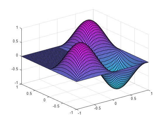
The Laplace operator is self-adjoint and negative definite, that is, only real negative eigenvalues $$\lambda$$ exist. There is a maximal (negative) discrete eigenvalue, the corresponding eigenfunction $$u$$ is called the ground state. In this example, $$\Omega$$ is an L-shaped region, and the ground state associated with this region is the L-shaped membrane that is the MATLAB® logo.

Nine-Point Finite Difference Approximation

The simplest approach to the eigenvalue problem is to approximate the Laplacian $$\Delta u$$ by a finite difference approximation (a stencil) on a square grid of points with distances hx in $$x$$ direction and distances hy in $$y$$ direction. In this example, approximate $$\Delta u$$ with a sum S_h of nine regular grid points around the midpoint $$(x,y)$$. The unknowns are the weights $$a_{-1-1},\dots ,a_{11}$$.

syms u(x,y) Eps a11 a10 a1_1 a01 a00 a0_1 a_11 a_10 a_1_1
syms hx hy positive
S_h = a_11 * u(x - Eps*hx,y + Eps*hy) +...
      a01  * u(x,y + Eps*hy) +...
      a11  * u(x + Eps*hx,y + Eps*hy) +... 
      a_10 * u(x - Eps*hx,y) +... 
      a00  * u(x,y) +... 
      a10  * u(x + Eps*hx,y) +...
      a_1_1* u(x - Eps*hx,y - Eps*hy) +...
      a0_1 * u(x,y - Eps*hy) +...
      a1_1 * u(x + Eps*hx,y - Eps*hy);

Use the symbolic parameter Eps to sort the expansion of this expression by powers of hx and hy. Knowing the weights, you can approximate the Laplacian by setting Eps = 1.

t = taylor(S_h, Eps, 'Order', 7);

Use the coeffs function to extract their coefficients of terms with the same powers of Eps. Each coefficient is an expression containing powers of hx, hy, and derivatives of u with respect to $$x$$ and $$y$$. Since S_h represents $$u_{xx}+u_{yy}$$, the coefficients of all other derivatives of u must be zero. Extract the coefficients by replacing all derivatives of u, except $$u_{xx}$$ and $$u_{yy}$$, by 0. Replace $$u_{xx}$$ and $$u_{yy}$$ by 1. This reduces the Taylor expansion to the coefficient you want to compute, and leads to the following six linear equations.

C = formula(coeffs(t, Eps, 'All'));
eq0  = subs(C(7),u(x,y),1) == 0;
eq11 = subs(C(6),[diff(u,x),diff(u,y)],[1,0]) == 0;
eq12 = subs(C(6),[diff(u,x),diff(u,y)],[0,1]) == 0;
eq21 = subs(C(5),[diff(u,x,x),diff(u,x,y),diff(u,y,y)],[1,0,0]) == 1;
eq22 = subs(C(5),[diff(u,x,x),diff(u,x,y),diff(u,y,y)],[0,1,0]) == 0;
eq23 = subs(C(5),[diff(u,x,x),diff(u,x,y),diff(u,y,y)],[0,0,1]) == 1;

Since there are nine unknown weights in S_h, add further equations by requiring that all third-order derivatives of u are 0.

eq31 = subs(C(4),[diff(u,x,x,x),diff(u,x,x,y),diff(u,x,y,y),diff(u,y,y,y)], [1,0,0,0]) == 0;
eq32 = subs(C(4),[diff(u,x,x,x),diff(u,x,x,y),diff(u,x,y,y),diff(u,y,y,y)], [0,1,0,0]) == 0;
eq33 = subs(C(4),[diff(u,x,x,x),diff(u,x,x,y),diff(u,x,y,y),diff(u,y,y,y)], [0,0,1,0]) == 0;
eq34 = subs(C(4),[diff(u,x,x,x),diff(u,x,x,y),diff(u,x,y,y),diff(u,y,y,y)], [0,0,0,1]) == 0;

Solve the resulting ten equations for the nine unknown weights. Use ReturnConditions to find all solutions including arbitrary parameters.

[a11,a10,a1_1,a01,a00,a0_1,a_11,a_10,a_1_1,parameters,conditions] = ...
    solve([eq0,eq11,eq12,eq21,eq22,eq23,eq31,eq32,eq33,eq34], ...
          [a11,a10,a1_1,a01,a00,a0_1,a_11,a_10,a_1_1], ...
          'ReturnConditions',true);

expand([a_11,a01,a11;...
        a_10,a00,a01;...
        a1_1,a0_1,a_1_1])

ans = 
$$\left(\begin{array}{ccc}z& \frac{1}{{\mathrm{hy}}^2}-2\hspace{0.17em}z& z\\ \frac{1}{{\mathrm{hx}}^2}-2\hspace{0.17em}z& 4\hspace{0.17em}z-\frac{2}{{\mathrm{hx}}^2}-\frac{2}{{\mathrm{hy}}^2}& \frac{1}{{\mathrm{hy}}^2}-2\hspace{0.17em}z\\ z& \frac{1}{{\mathrm{hy}}^2}-2\hspace{0.17em}z& z\end{array}\right)$$

parameters

parameters = $$z$$

Use the subs function to replace the weights by their computed values.

C = simplify(subs(C));

The expressions C(7), C(6), and C(4) containing the 0th, 1st, and 3rd derivatives of u vanish.

[C(7), C(6), C(4)]

ans = $$\left(\begin{array}{ccc}0& 0& 0\end{array}\right)$$

The expression C(5) is the Laplacian of u.

C(5)

ans = 
$$\frac{{\partial }^2}{\partial x^2}\mathrm{ }u\left(x,y\right)+\frac{{\partial }^2}{\partial y^2}\mathrm{ }u\left(x,y\right)$$

Thus, with the values of the weights computed above, the stencil S_h approximates the Laplacian up to order hx^2, hy^2 for any values of the arbitrary parameter z, provided that z is chosen to be of order O(1/hx^2,1/hy^2).

Terms Containing Fourth and Higher Order Derivatives

Although the solution contains a free parameter z, the expression C(3) containing the fourth-order derivatives of u cannot be turned into zero by a suitable choice of z. Another option is to turn it into a multiple of the square of the Laplace operator.

syms d
Laplace = @(u) laplacian(u,[x,y]);
expand(d*Laplace(Laplace(u)))

ans(x, y) = 
$$d\hspace{0.17em}\frac{{\partial }^4}{\partial x^4}\mathrm{ }u\left(x,y\right)+2\hspace{0.17em}d\hspace{0.17em}\frac{{\partial }^2}{\partial y^2}\mathrm{ }\frac{{\partial }^2}{\partial x^2}\mathrm{ }u\left(x,y\right)+d\hspace{0.17em}\frac{{\partial }^4}{\partial y^4}\mathrm{ }u\left(x,y\right)$$

Pick different derivatives of u in C(3), and equate their coefficients with the corresponding terms.

subs(C(3),[diff(u,x,x,x,x),diff(u,x,x,y,y),diff(u,y,y,y,y)],[1,0,0]) == d

ans = 
$$\frac{{\mathrm{hx}}^2}{12}=d$$

subs(C(3),[diff(u,x,x,x,x),diff(u,x,x,y,y),diff(u,y,y,y,y)],[0,1,0]) == 2*d

ans = $${\mathrm{hx}}^2\hspace{0.17em}{\mathrm{hy}}^2\hspace{0.17em}z=2\hspace{0.17em}d$$

subs(C(3),[diff(u,x,x,x,x),diff(u,x,x,y,y),diff(u,y,y,y,y)],[0,0,1]) == d

ans = 
$$\frac{{\mathrm{hy}}^2}{12}=d$$

Therefore, you can choose d = hx^2/12 = hy^2/12 and z = 2*d/(hx^2*hy^2), implying that hx = hy and z = 1/(6*hx*hy). Hence, the stencil S_h approximates a modified Laplacian on a square grid with hx = hy = h.

syms h
hx = h;
hy = h;
d = h^2/12;

Replace hx and hy by h.

C = subs(C);

Replace z by its value, 1/(6*h^2). Because z does not exist in the MATLAB workspace, you can access it only as the value stored in the parameters array.

C = subs(C,parameters,1/(6*h^2));

Verify the formula (1).

simplify(C(3) - d*Laplace(Laplace(u)))

ans(x, y) = $$0$$

Now, consider the third-order terms in hx, hy.

simplify(C(2))

ans = $$0$$

Since no such terms exist in the expansion of the stencil, the term $$O(h^3)$$ in (1) is in fact of order $$O(h^4)$$. Consider the fourth-order terms of the stencil.

factor(simplify(C(1)))

ans = 
$$\left(\begin{array}{cccccc}\frac{1}{360}& h& h& h& h& \frac{{\partial }^6}{\partial x^6}\mathrm{ }u\left(x,y\right)+5\hspace{0.17em}\frac{{\partial }^2}{\partial y^2}\mathrm{ }\frac{{\partial }^4}{\partial x^4}\mathrm{ }u\left(x,y\right)+5\hspace{0.17em}\frac{{\partial }^4}{\partial y^4}\mathrm{ }\frac{{\partial }^2}{\partial x^2}\mathrm{ }u\left(x,y\right)+\frac{{\partial }^6}{\partial y^6}\mathrm{ }u\left(x,y\right)\end{array}\right)$$

Check if these terms can be identified with yet another power of the Laplace operator. However, comparison with

Laplace(Laplace(Laplace(u)))

ans(x, y) = 
$$\frac{{\partial }^6}{\partial x^6}\mathrm{ }u\left(x,y\right)+3\hspace{0.17em}\frac{{\partial }^2}{\partial y^2}\mathrm{ }\frac{{\partial }^4}{\partial x^4}\mathrm{ }u\left(x,y\right)+3\hspace{0.17em}\frac{{\partial }^4}{\partial y^4}\mathrm{ }\frac{{\partial }^2}{\partial x^2}\mathrm{ }u\left(x,y\right)+\frac{{\partial }^6}{\partial y^6}\mathrm{ }u\left(x,y\right)$$

shows that the expressions of order $$O(h^4)$$ cannot be identified as some multiple of the third power of the Laplace operator because the coefficients cannot be matched.

Summary

For a square grid with distance h between neighboring grid points and the above choices of the weights, you get:

Use this expansion for the numeric approach to the eigenvalue problem $$\Delta u=\lambda u$$. Add some multiple of $${\Delta }^{2}u={\lambda }^{2}u$$ to the eigenvalue equation.

The left side of this equation is well approximated by the stencil $$S_h$$. Thus, using (2), a numerical eigenvalue $$\mu$$ of the stencil satisfying $$S_{h}u=\mu u$$ must be an approximation of the eigenvalue $$\lambda$$ of the Laplace operator with

For given $$\mu$$, solve for $$\lambda$$ to obtain a better approximation of the Laplace eigenvalue. Note that in the solution of the quadratic equation in $$\lambda$$ the correct sign of the square root is given by the requirement that $$\lambda \to \mu$$ for $$h\to 0$$.

Using Symbolic Matrices to Solve the Eigenvalue Problem

Consider an L-shaped region $$\Omega$$ consisting of three unit squares.

Define the coordinate values of the corners of the region.

xmin =-1;
xmax = 1; 
ymin =-1; 
ymax = 1;

Consider a square grid consisting of an odd number Nx=2*nx-1 of grid points in x direction and an odd number Ny=2*ny-1 of grid points in y direction.

nx = 6; 
Nx = 2*nx-1; 
hx = (xmax-xmin)/(Nx-1);

ny = 6; 
Ny = 2*ny-1; 
hy = (ymax-ymin)/(Ny-1);

Create an Ny-by- Nx symbolic matrix $$u$$. Its entries u(i,j) represent the values u(xmin + (j - 1)*hx,ymin + (i - 1)*hy) of the solution u(x,y) of the eigenvalue problem $$\Delta u=\lambda u$$.

u = sym('u',[Ny,Nx]);

The boundaries of $$\Omega$$ correspond to the following indices:

u(:,1) = 0;      % left boundary
u(1,:) = 0;      % lower boundary
u(1:ny,Nx) = 0;  % right boundary, upper part
u(ny:Ny,nx) = 0; % right boundary, lower part
u(Ny,1:nx) = 0;  % upper boundary, left part
u(ny,nx:Nx) = 0; % upper boundary, right part

The region with $$0<x\le 1$$ and $$0<y\le 1$$ does not belong to $$\Omega$$. Set the corresponding matrix entries (i = ny + 1:Ny, j = nx + 1:Nx) to zero. They play no further role and will be ignored.

u(ny + 1:Ny,nx + 1:Nx) = 0;

The unknowns of the problem are the following matrix entries:

u

u = 
$$\left(\begin{array}{ccccccccccc}0& 0& 0& 0& 0& 0& 0& 0& 0& 0& 0\\ 0& u_{2,2}& u_{2,3}& u_{2,4}& u_{2,5}& u_{2,6}& u_{2,7}& u_{2,8}& u_{2,9}& u_{2,10}& 0\\ 0& u_{3,2}& u_{3,3}& u_{3,4}& u_{3,5}& u_{3,6}& u_{3,7}& u_{3,8}& u_{3,9}& u_{3,10}& 0\\ 0& u_{4,2}& u_{4,3}& u_{4,4}& u_{4,5}& u_{4,6}& u_{4,7}& u_{4,8}& u_{4,9}& u_{4,10}& 0\\ 0& u_{5,2}& u_{5,3}& u_{5,4}& u_{5,5}& u_{5,6}& u_{5,7}& u_{5,8}& u_{5,9}& u_{5,10}& 0\\ 0& u_{6,2}& u_{6,3}& u_{6,4}& u_{6,5}& 0& 0& 0& 0& 0& 0\\ 0& u_{7,2}& u_{7,3}& u_{7,4}& u_{7,5}& 0& 0& 0& 0& 0& 0\\ 0& u_{8,2}& u_{8,3}& u_{8,4}& u_{8,5}& 0& 0& 0& 0& 0& 0\\ 0& u_{9,2}& u_{9,3}& u_{9,4}& u_{9,5}& 0& 0& 0& 0& 0& 0\\ 0& u_{10,2}& u_{10,3}& u_{10,4}& u_{10,5}& 0& 0& 0& 0& 0& 0\\ 0& 0& 0& 0& 0& 0& 0& 0& 0& 0& 0\end{array}\right)$$

The interior points of the region $$\Omega \setminus \partial \Omega$$ correspond to the indices $$(i,j)$$ that contain the unknown values $$u(i,j)$$ of the problem. Collect these unknowns in a vector vars.

[I,J] = find(u~=0);
vars = u(u~=0);

Associate a symbolic expression (given by the stencil derived in the first part of this example) with each index (that is, with each unknown).

n = length(vars);
Lu = sym(zeros(n,1));
for k=1:n
   i = I(k);
   j = J(k);
   Lu(k) =   1/6*u(i+1,j-1) +  2/3*u(i+1,j) + 1/6*u(i+1,j+1) ...
           + 2/3*u( i ,j-1) - 10/3*u( i ,j) + 2/3*u( i ,j+1) ...
           + 1/6*u(i-1,j-1) +  2/3*u(i-1,j) + 1/6*u(i-1,j+1); 
end
Lu = Lu/hx^2;

Because this expression is linear in the unknown elements of u (stored in vars), you can treat it as a matrix acting on the vector vars.

S_h = jacobian(Lu, vars);

You can treat S_h as a matrix approximation of the Laplace operator. Compute its eigenvectors and eigenvalues.

[V,D] = eig(vpa(S_h));

The three maximal eigenvalues are given by the first diagonal elements of D.

[D(1,1), D(2,2), D(3,3)]

ans = $$\left(\begin{array}{ccc}-9.5214641572625960021345709535953& -14.431096242107969492574666743957& -18.490392088545609858994660377955\end{array}\right)$$

Since for this approximation you used a grid with a small number of points, only the leading digits of the eigenvalues are correct.

The third highest eigenvalue of the Laplace operator on the L-shaped region $$\Omega$$ is known exactly. The exact eigenfunction of the Laplace operator is the function $$u(x,y)=\sin (\pi x)\sin (\pi y)$$ associated with the (exact) eigenvalue $$-2{\pi }^2=-19.7392...$$. Indeed, using equation (3) above, you can derive a better approximation of the Laplace eigenvalue $$\lambda$$ from the stencil eigenvalue $$\mu$$:

mu = D(3,3)

mu = $$-18.490392088545609858994660377955$$

lambda = 2*mu / (sqrt(1 + mu*hx^2/3) + 1)

lambda = $$-19.796765119155672176257649532142$$

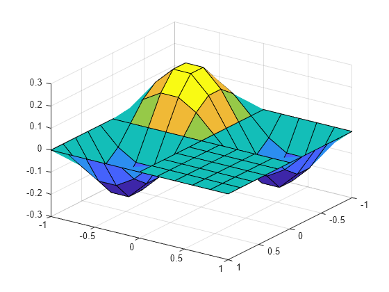
Plot the eigenfunction associated with the third highest eigenvalue.

v = V(:,3);
for k=1:n
  u(I(k),J(k)) = v(k);
end
u = double(u);
surf(xmin:hx:xmax,ymin:hy:ymax,u');
view(125, 30);

Using Double-Precision Matrices to Solve the Eigenvalue Problem

When you use symbolic matrices, increasing the number of grid points drastically is not recommended because symbolic computations are significantly slower than numerical computations with MATLAB double-precision matrices. This part of the example demonstrates how to use sparse double arithmetic which allows to refine the numerical grid. The L-shaped region $$\Omega$$ is set up the same way as before. Instead of denoting the interior points by symbolic unknowns, initialize the grid values u by ones and define $$\Omega$$ by setting the values of boundary points and exterior points to zero. Instead of defining a symbolic expression for each interior point and computing the stencil as the Jacobian, set up the stencil matrix directly as a sparse matrix.

xmin =-1; 
xmax = 1; 
ymin =-1; 
ymax = 1;

nx = 30; 
Nx = 2*nx-1; 
hx = (xmax-xmin)/(Nx-1);

ny = 30; 
Ny = 2*ny-1; 
hy = (ymax-ymin)/(Ny-1);

u = ones(Ny,Nx); 
u(:,1) = 0;      % left boundary
u(1:ny,Nx) = 0;  % right boundary, upper part
u(ny:Ny,nx) = 0; % right boundary, lower part
u(1,:) = 0;      % lower boundary
u(Ny,1:nx) = 0;  % upper boundary, left part
u(ny,nx:Nx) = 0; % upper boundary, right part
u(ny + 1:Ny,nx + 1:Nx) = 0;

[I,J] = find(u ~= 0);
n = length(I);
S_h = sparse(n,n);
for k=1:n 
  i = I(k);
  j = J(k);
  S_h(k,I==i+1 & J==j+1)=  1/6;
  S_h(k,I==i+1 & J== j )=  2/3;
  S_h(k,I==i+1 & J==j-1)=  1/6;
  S_h(k,I== i  & J==j+1)=  2/3;
  S_h(k,I== i  & J== j )=-10/3;
  S_h(k,I== i  & J==j-1)=  2/3;
  S_h(k,I==i-1 & J==j+1)=  1/6;
  S_h(k,I==i-1 & J== j )=  2/3;
  S_h(k,I==i-1 & J==j-1)=  1/6;
end
S_h = S_h./hx^2;

Here, S_h is the (sparse) stencil matrix. Use eigs that handles sparse matrices to compute the three largest eigenvalues.

[V,D] = eigs(S_h,3,'la');

The three maximal eigenvalues are the first diagonal elements of D.

[D(1,1), D(2,2), D(3,3)]

ans = 1×3

   -9.6493  -15.1742  -19.7006

D(3,3) approximates the exact eigenvalue $$-2{\pi }^2=-19.7392088...$$. Using the equation (3) above, derive a more accurate approximation of the Laplace eigenvalue $$\lambda$$ from the stencil eigenvalue $$\mu$$.

mu = D(3,3)

mu = 
-19.7006

lambda = 2*mu / (sqrt(1 + mu*hx^2/3) + 1)

lambda = 
-19.7393

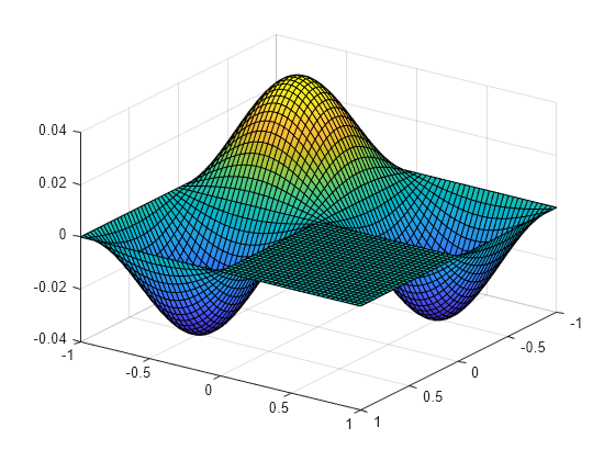
Plot the eigenfunction associated with the third highest eigenvalue.

v = V(:,3);
for k=1:n
  u(I(k),J(k)) = v(k);
end
surf(xmin:hx:xmax, ymin:hy:ymax,u');
view(125, 30);

Note that the MATLAB membrane function computes the eigenfunctions of the Laplace operator by different methods.

membrane(3, nx - 1, 8, 8);