Detect Irregularities in 3-D Volumetric Lung CT Data Using PatchCore Anomaly Detector

Since R2026a

This example uses:

This example shows how to detect irregularities in 3-D volumetric computed tomography (CT) data of lungs by using a PatchCore anomaly detector that uses a pretrained ResNet-101 model as the backbone.

PatchCore is an anomaly detection method that focuses on identifying unusual patterns in images by analyzing local patches rather than the entire image. It extracts features from these patches using a pretrained backbone deep learning model and selects a representative subset to capture normal patterns efficiently. During inference, the detector compares new image patches to the representative subset to compute anomaly scores, and then aggregates the scores to determine the presence of anomalies. In medical imaging, PatchCore is particularly useful for detecting subtle abnormalities in scans, such as identifying rare diseases or early-stage tumors, because it can focus on localized deviations from normal tissue patterns.

Download Data Set

This example uses the SPIE Lung Nodule Classification Data Set [1], which contains both benign and malignant lung CT volume data. The train and test data sets include multiple volume CT scans, each represented as a series of DICOM images. This example uses 10 training scans and 17 test scans from the SPIE Lung Nodule Classification Data Set. The training data set has been preprocessed for faster execution.

Specify the location of the data set. Download the data set and unzip the contents of the folder into the specified location using the helperDownloadLungDefectDetectorModelDataset helper function. The helper function is attached to this example as a supporting file.

dataSetDownloadURL = "https://ssd.mathworks.com/supportfiles/vision/data/LungDefectDetectorModelDataset.zip";
dataDir = fullfile(pwd,"LungDefectDetectorModelDataset");
helperDownloadLungDefectDetectorModelDataset(dataSetDownloadURL,dataDir)

Downloading LungDefectDetectorModel data set.
This can take several minutes to download and unzip...
Done.

Prepare Data for Training

The training data set contains preprocessed data of 10 benign or healthy lung CT scans. Each lung CT volume in the training data set has been preprocessed using these steps.

Align the lung CT volume from the series of DICOM files to the orientation suitable for the pretrained network to perform lung segmentation.
Preprocess the volume by using the helperPreprocessVolume helper function. The helper function is attached to this example as a supporting file. The helperPreprocessVolume function clips the intensity range of the volume to the range [-1024, 600] Hounsfield units (HU), and crops and resizes the volume to match the input size of the pretrained network for lung segmentation.
Segment the left and right lungs using the pretrained LungMask Unet R231 deep learning model by using the helperSegmentLungMask helper function. The helperSegmentLungMask helper function is attached to this example as a supporting file. To decrease the required computational time, the helperSegmentLungMask function performs inference on the slices of a volume in batches. Obtain the segmentation masks by postprocessing the network output by using the helperPostprocessMask helper function. The helperPostprocessMask helper function is attached to this example as a supporting file. The helperPostprocessMask function removes the small connected components, fills holes, and reshapes the segmented mask to the original size of the volume.
Generate 2-D views for both the right and left lungs in the axial, sagittal, and coronal directions by performing maximum intensity projection (MIP) using the helperComputeMaximumIntensityProjections helper function. The helperComputeMaximumIntensityProjections helper function is attached to this example as a supporting file. Store the six projection images for each lung CT volume in separate folders named la (left axial), ls (left sagittal), lc (left coronal), ra (right axial), rs (right sagittal), and rc (right coronal). The helperComputeMaximumIntensityProjections function clips the intensity values to the range [-800, 200] HU, normalizes the truncated 3-D volume using min-max normalization, and applies MIP to generate the six projections. This approach ensures that the MIP performed after truncated normalization retains only the most shaded pixels within the intensity region of interest on the projection plane, facilitating detailed examination of potentially abnormal structures within the 3-D lung stack on that plane.

You can perform these preprocessing steps on a sample training image.

Load sample lung CT volume data from the training data set.

sampleTrainVol = fullfile(dataDir,"data","trainSample","LUNGx-CT005");
medVolInp = medicalVolume(sampleTrainVol);

Display the sample volume.

volshow(medVolInp,RenderingStyle="GradientOpacity")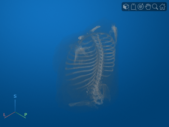

Extract the voxels, and determine the size of the volume.

volData = medVolInp.Voxels;
origVolSize = size(volData);

Align the lung CT volume from the series of DICOM files to the orientation suitable for the pretrained network to perform lung segmentation.

rotationAxis = [0 0 1];
volAligned = imrotate3(volData,90,rotationAxis);

Preprocess the volume by using the helperPreprocessVolume helper function.

[volDataPreprocessed,bboxMatrix] = helperPreprocessVolume(volAligned);

Segment the left and right lungs using the pretrained LungMask Unet R231 deep learning model by using the helperSegmentLungMask helper function.

maskVol = helperSegmentLungMask(volDataPreprocessed);

Obtain the segmentation masks by postprocessing the network output by using the helperPostprocessMask helper function.

outMaskVol = helperPostprocessMask(maskVol,origVolSize,bboxMatrix);

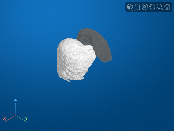
Display the output mask.

volshow(outMaskVol)

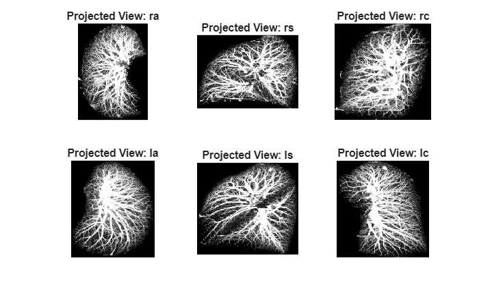
Generate 2-D views for both the right and left lungs in the axial, sagittal, and coronal directions by performing maximum intensity projection (MIP) using the helperComputeMaximumIntensityProjections helper function.

[imgArrayPostMIP,maskArrayPostMIP] = helperComputeMaximumIntensityProjections(outMaskVol,volAligned);

Specify the projection names.

projectionNames = ["ra","rs","rc","la","ls","lc"];
numViews = length(projectionNames);

Display the projections.

tiledlayout(2,3)
for viewIdx = 1:size(imgArrayPostMIP,2)
    nexttile
    imshow(imgArrayPostMIP{viewIdx})
    title("Projected View: " + projectionNames(viewIdx))
end

Define Network Architecture

Create the PatchCore network by using the patchCoreAnomalyDetector object, and specify resnet101 as the backbone.

patchcore = patchCoreAnomalyDetector(Backbone="resnet101");

Specify the network input size.

networkInputSize = [224 224];

Train Network

Set the global random state to "default" to ensure reproducibility.

rng("default")

Train the PatchCore network on the preprocessed training images for all the six specified projection directions by using the trainPatchCoreAnomalyDetector function. Specify the compression ratio as 1 as the training data is limited.

sourceTrainProjections = fullfile(dataDir,"data","projectionsTrain");
trainedDetectors = cell(1,numViews);

for i = 1:numViews
    selectedView = projectionNames(i);
    trainFolder = fullfile(sourceTrainProjections,selectedView);
    dsTrain = imageDatastore(trainFolder);
    dsTrain.Labels = zeros(1,length(dsTrain.Files));
    dsTrainFinal = transform(dsTrain,@(x)imresize(repmat(x,[1 1 3]),networkInputSize,"nearest",Antialiasing=false));
    detector = trainPatchCoreAnomalyDetector(dsTrainFinal,patchcore,CompressionRatio=1,MiniBatchSize=1,Verbose=false);
    trainedDetectors{i} = detector;
end

Detect Irregularities in Test Data

Create the test volume datastore and the ground truth labels for each of the test volumes by using the helperCreateMedicalVolumeArray helper function. The helperCreateMedicalVolumeArray helper function is attached to this example as a supporting file. The helperCreateMedicalVolumeArray function reads each of the test DICOM directories as a medicalVolume object and generates the ground truth label for that volume after extracting label information from the gt.txt file.

sourceDirTest = fullfile(dataDir,"data","test");
[outMedVolArrTest,gtLabelsArrTest] = helperCreateMedicalVolumeArray(sourceDirTest);

Started processing to create medical volume datastore ...
Operation completed for dicom folder 1 of 17 (5.88% complete)
Operation completed for dicom folder 2 of 17 (11.76% complete)
Operation completed for dicom folder 3 of 17 (17.65% complete)
Operation completed for dicom folder 4 of 17 (23.53% complete)
Operation completed for dicom folder 5 of 17 (29.41% complete)
Operation completed for dicom folder 6 of 17 (35.29% complete)
Operation completed for dicom folder 7 of 17 (41.18% complete)
Operation completed for dicom folder 8 of 17 (47.06% complete)
Operation completed for dicom folder 9 of 17 (52.94% complete)
Operation completed for dicom folder 10 of 17 (58.82% complete)
Operation completed for dicom folder 11 of 17 (64.71% complete)
Operation completed for dicom folder 12 of 17 (70.59% complete)
Operation completed for dicom folder 13 of 17 (76.47% complete)
Operation completed for dicom folder 14 of 17 (82.35% complete)
Operation completed for dicom folder 15 of 17 (88.24% complete)
Operation completed for dicom folder 16 of 17 (94.12% complete)
Operation completed for dicom folder 17 of 17 (100.00% complete)
Done.

Preprocess the test data, and generate 2-D views for both the right and left lungs in the axial, sagittal, and coronal directions, similar to the training data. Obtain the anomaly score for each of the six projections in the test data using the trained PatchCore network by using the predict function. Generate the anomaly score heatmap for the projection views by using the anomalyMap function. From the predicted anomaly scores of the six projections in each volume, assign the maximum value as the anomaly score for that volume.

numTestVols = size(outMedVolArrTest,1);

mask3dArrTest = cell(1,numTestVols);
mask2dProjectionsTest = cell(1,numTestVols);
img2dProjectionsTest = cell(1,numTestVols);
scoresArrTest = [];
anomapsArrTest = cell(1,numTestVols);

for idx = 1:numTestVols

    %---------------- Segmentation of lungs ----------------------------
    % Load the medical volume data
    medVolInp = outMedVolArrTest{idx};
    volData = medVolInp.Voxels;
    origVolSize = size(volData);

    % Align volume data
    rotationAxis = [0 0 1];
    volAligned = imrotate3(volData,90,rotationAxis);

    % Preprocess volume data
    [volDataPreprocessed,bboxMatrix] = helperPreprocessVolume(volAligned);

    % Segment lungs
    maskVol = helperSegmentLungMask(volDataPreprocessed);

    % Postprocess mask
    outMask = helperPostprocessMask(maskVol,origVolSize,bboxMatrix);
    mask3dArrTest{idx} = outMask;

    %------------------- Generate projections ----------------------------
    [imgArrayPostMIP,maskArrayPostMIP] = helperComputeMaximumIntensityProjections(outMask,volAligned);
    img2dProjectionsTest{idx} = imgArrayPostMIP;
    mask2dProjectionsTest{idx} = maskArrayPostMIP;

    %----------------- Inference ----------------------------------------
    outAnoMapPerVol = cell(1,numViews);
    outScoresPerVol = [];

    for viewIdx = 1:numViews
        selectedView = projectionNames(viewIdx);
        
        % Load the trained detector for selected view
        detector = trainedDetectors{viewIdx};

        % 2-D view from test data
        testImage = imgArrayPostMIP{viewIdx};
        testImage = imresize(repmat(testImage,[1 1 3]),networkInputSize,"nearest",Antialiasing=false);

        % Predict score and anomaly heatmap
        score = predict(detector,testImage);        
        anomalyHeatMap = anomalyMap(detector,testImage);

        outScoresPerVol = [outScoresPerVol; score];
        outAnoMapPerVol{viewIdx} = anomalyHeatMap;
    end

    % Take the maximum of all the detection scores from the projection views
    maxi = max(outScoresPerVol,[],"all");
    scoresArrTest = [scoresArrTest; maxi];

    % Store the 2-D anomaly maps
    anomapsArrTest{idx} = outAnoMapPerVol;

    progress = (idx/numTestVols)*100;
    fprintf("Completed inference for Test Volume %d of %d (%.2f%% complete)\n",idx,numTestVols,progress)
end

Completed inference for Test Volume 1 of 17 (5.88% complete)
Completed inference for Test Volume 2 of 17 (11.76% complete)
Completed inference for Test Volume 3 of 17 (17.65% complete)
Completed inference for Test Volume 4 of 17 (23.53% complete)
Completed inference for Test Volume 5 of 17 (29.41% complete)
Completed inference for Test Volume 6 of 17 (35.29% complete)
Completed inference for Test Volume 7 of 17 (41.18% complete)
Completed inference for Test Volume 8 of 17 (47.06% complete)
Completed inference for Test Volume 9 of 17 (52.94% complete)
Completed inference for Test Volume 10 of 17 (58.82% complete)
Completed inference for Test Volume 11 of 17 (64.71% complete)
Completed inference for Test Volume 12 of 17 (70.59% complete)
Completed inference for Test Volume 13 of 17 (76.47% complete)
Completed inference for Test Volume 14 of 17 (82.35% complete)
Completed inference for Test Volume 15 of 17 (88.24% complete)
Completed inference for Test Volume 16 of 17 (94.12% complete)
Completed inference for Test Volume 17 of 17 (100.00% complete)

Evaluate Network on Test Data

Calculate the optimal anomaly threshold by using the anomalyThreshold function. Specify the first two input arguments as the ground truth labels gtLabelsArrTest and the predicted anomaly scores scoresArrTest for the test data set. Specify the third input argument as 1 because true positive anomaly images have a label of 1. The anomalyThreshold function returns the optimal threshold value, as a scalar, and the receiver operating characteristic (ROC) curve for the detector, as an rocmetrics object.

[threshold,roc] = anomalyThreshold(gtLabelsArrTest,scoresArrTest,1);

Predict class labels for each test set volume by comparing the predicted anomaly score to the threshold value.

predLabels = scoresArrTest > threshold;

Evaluate the anomaly detector by calculating performance metrics using the evaluateAnomalyDetection function. The evaluateAnomalyDetection function calculates several metrics that evaluate the accuracy, precision, sensitivity, and specificity of the detector for the test data set.

metrics = evaluateAnomalyDetection(predLabels,gtLabelsArrTest,1);

Evaluating anomaly detection results
------------------------------------
* Finalizing... Done.
* Data set metrics:

    GlobalAccuracy    MeanAccuracy    Precision    Recall     Specificity    F1Score    FalsePositiveRate    FalseNegativeRate
    ______________    ____________    _________    _______    ___________    _______    _________________    _________________

       0.76471          0.75714        0.71429     0.71429        0.8        0.71429           0.2                0.28571

Calculate the confusion matrix and the classification accuracy for the test data set.

M = metrics.ConfusionMatrix{:,:};
figure
confusionchart(M,["Normal","Anomaly"])
acc = sum(diag(M))/sum(M,"all");
title("Accuracy: " + acc)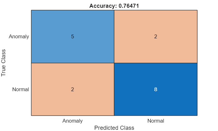

Plot the ROC curve by using the plot function. The ROC curve illustrates the performance of the classifier for a range of possible threshold values. Each point on the ROC curve represents the false positive rate (x-coordinate) and true positive rate (y-coordinate) when you classify the calibration set images using a different threshold value. The solid blue line represents the ROC curve. The area under the ROC curve (AUC) metric indicates classifier performance, with a perfect classifier corresponding to the maximum ROC AUC of 1.

figure
plot(roc)
title("ROC AUC: " + roc.AUC)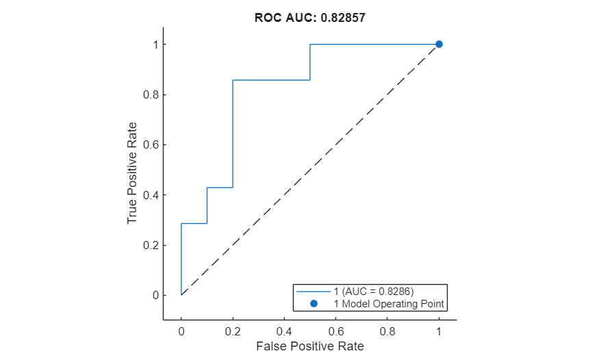

Visualize 2-D Heatmap

Compute the maximum anomaly score for each projection across the test data set by using the getMaxValPerView helper function defined at the end of this example.

maxPerView = getMaxValPerView(anomapsArrTest);
% Reorder the projection views for better visualization
projectionNames = ["ra","la","rs","ls","rc","lc"];
maxPerView = [maxPerView(1) maxPerView(4) maxPerView(2) maxPerView(5) maxPerView(3) maxPerView(6)];

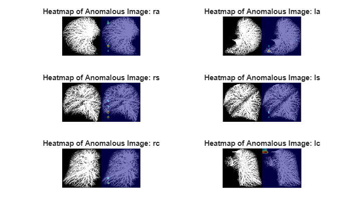
Select a test volume that is correctly classified as anomalous.

idxTruePositive = find(gtLabelsArrTest & predLabels);
selectedIdxTP = idxTruePositive(end);
imagesSampleTest = img2dProjectionsTest{selectedIdxTP};
imagesSampleTest = {imagesSampleTest{1} imagesSampleTest{4} imagesSampleTest{2} imagesSampleTest{5} imagesSampleTest{3} imagesSampleTest{6}};
anomalyMaps2DSampleTest = anomapsArrTest{selectedIdxTP};
anomalyMaps2DSampleTest = {anomalyMaps2DSampleTest{1} anomalyMaps2DSampleTest{4} anomalyMaps2DSampleTest{2} anomalyMaps2DSampleTest{5} anomalyMaps2DSampleTest{3} anomalyMaps2DSampleTest{6}};

To compare anomaly scores observed across the entire test data set, normalize the anomaly map based on the maximum score for each projection. Display the 2-D views of the chosen test volume with the heatmap overlaid by using the anomalyMapOverlay function

figure
tiledlayout(3,2)
for idx = 1:numViews
    sampleImage = imagesSampleTest{idx};
    sampleImage = imresize(sampleImage,networkInputSize);
    anomalyHeatMap = anomalyMaps2DSampleTest{idx};
    displayRange = [maxPerView(idx)*0.9 maxPerView(idx)];
    heatMapImage = anomalyMapOverlay(sampleImage,anomalyHeatMap,Blend="equal",MapRange=displayRange);
    nexttile
    montage({sampleImage heatMapImage})
    title("Heatmap of Anomalous Image: " + projectionNames{idx})
end

Similarly, select a test volume that is correctly classified as normal, and display it with the heatmap overlaid by using the anomalyMapOverlay function.

idxTrueNegative  = find(~(gtLabelsArrTest | predLabels));
selectedIdxTN = idxTrueNegative(end);
imagesSampleTest = img2dProjectionsTest{selectedIdxTN};
imagesSampleTest = {imagesSampleTest{1} imagesSampleTest{4} imagesSampleTest{2} imagesSampleTest{5} imagesSampleTest{3} imagesSampleTest{6}};
anomalyMaps2DSampleTest = anomapsArrTest{selectedIdxTN};
anomalyMaps2DSampleTest = {anomalyMaps2DSampleTest{1} anomalyMaps2DSampleTest{4} anomalyMaps2DSampleTest{2} anomalyMaps2DSampleTest{5} anomalyMaps2DSampleTest{3} anomalyMaps2DSampleTest{6}};

figure
tiledlayout(3,2)
for idx = 1:numViews
    sampleImage = imagesSampleTest{idx};
    sampleImage = imresize(sampleImage,networkInputSize);
    anomalyHeatMap = anomalyMaps2DSampleTest{idx};
    displayRange = [maxPerView(idx)*0.9 maxPerView(idx)];
    heatMapImage = anomalyMapOverlay(sampleImage,anomalyHeatMap,Blend="equal",MapRange=displayRange);
    nexttile
    montage({sampleImage heatMapImage})
    title("Heatmap of Normal Image: " + projectionNames{idx})
end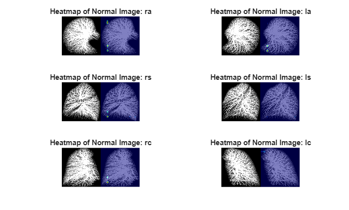

Supporting Functions

function maxScorePerView = getMaxValPerView(anomapsArrTest)
% This function returns a 1-by-6 vector containing the maximum anomaly
% score for each of the six projection views.

    numViews = 6;
    maxScorePerView = zeros(1,numViews);

    for viewIdx = 1:numViews
        scoresPerView = [];
        for i = 1:length(anomapsArrTest)
            scoresPerView = [scoresPerView; anomapsArrTest{i}{viewIdx}];
        end
        % Find the maximum value for the current direction
        maxScorePerView(viewIdx) = max(scoresPerView,[],"all");
    
    end
end

References

[1] Armato, Samuel G., Karen Drukker, Feng Li, et al. “LUNGx Challenge for Computerized Lung Nodule Classification.” Journal of Medical Imaging 3, no. 4 (2016): 044506. https://doi.org/10.1117/1.JMI.3.4.044506.

[2] Kim, Kyung-Su, Seong Je Oh, Ju Hwan Lee, and Myung Jin Chung. “3D Unsupervised Anomaly Detection and Localization through Virtual Multi-View Projection and Reconstruction: Clinical Validation on Low-Dose Chest Computed Tomography.” Preprint, arXiv, 2022. https://doi.org/10.48550/ARXIV.2206.13385.