Develop Visual SLAM Algorithm Using Unreal Engine Simulation

This example uses:

This example shows how to develop a visual Simultaneous Localization and Mapping (SLAM) algorithm using image data obtained from the Unreal Engine® simulation environment.

Visual SLAM is the process of calculating the position and orientation of a camera with respect to its surroundings while simultaneously mapping the environment. Developing a visual SLAM algorithm and evaluating its performance in varying conditions is a challenging task. One of the biggest challenges is generating the ground truth of the camera sensor, especially in outdoor environments. The use of simulation enables testing under a variety of scenarios and camera configurations while providing precise ground truth.

This example demonstrates the use of Unreal Engine simulation to develop a visual SLAM algorithm for either a monocular or a stereo camera in a parking scenario. For more information about the implementation of the visual SLAM pipelines, see the Monocular Visual Simultaneous Localization and Mapping example and the Stereo Visual Simultaneous Localization and Mapping example.

Set Up Scenario in Simulation Environment

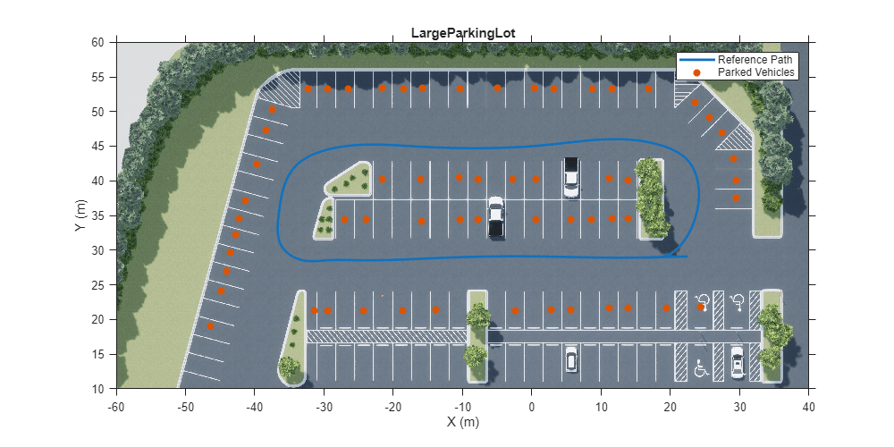
Use the Simulation 3D Scene Configuration block to set up the simulation environment. Select the built-in Large Parking Lot scene, which contains several parked vehicles. The visual SLAM algorithm matches features across consecutive images. To increase the number of potential feature matches, you can use the Parked Vehicles subsystem to add more parked vehicles to the scene. To specify the parking poses of the vehicles, use the helperAddParkedVehicle function. If you select a more natural scene, the presence of additional vehicles is not necessary. Natural scenes usually have enough texture and feature variety suitable for feature matching.

You can follow the Select Waypoints for Unreal Engine Simulation (Automated Driving Toolbox) example to interactively select a sequence of parking locations. You can use the same approach to select a sequence of waypoints and generate a reference trajectory for the ego vehicle. This example uses a recorded reference trajectory and parked vehicle locations.

% Load reference path
data = load("parkingLotReferenceData.mat");

% Set reference trajectory of the ego vehicle
refPosesX = data.refPosesX;
refPosesY = data.refPosesY;
refPosesT = data.refPosesT;

% Set poses of the parked vehicles
parkedPoses = data.parkedPoses;

% Display the reference path and the parked vehicle locations
sceneName = "LargeParkingLot";
hScene = figure;
helperShowSceneImage(sceneName);
hold on
plot(refPosesX(:,2), refPosesY(:,2), LineWidth=2, DisplayName='Reference Path');
scatter(parkedPoses(:,1), parkedPoses(:,2), [], 'filled', DisplayName='Parked Vehicles');
xlim([-60 40])
ylim([10 60])
hScene.Position = [100, 100, 1000, 500]; % Resize figure
legend
hold off

Figure contains an axes object. The axes object with title LargeParkingLot, xlabel X (m), ylabel Y (m) contains 3 objects of type image, line, scatter. These objects represent Reference Path, Parked Vehicles.

Open the model and add parked vehicles

modelName = 'GenerateImageDataOfParkingLot';
open_system(modelName);

Figure Video Viewer contains an axes object and other objects of type uiflowcontainer, uimenu, uitoolbar. The axes object contains an object of type image.

helperAddParkedVehicles(modelName, parkedPoses);

Set Up Ego Vehicle and Camera Sensor

Set up the ego vehicle moving along the specified reference path by using the Simulation 3D Vehicle with Ground Following block. The Camera Variant Subsystem contains two configurations of camera sensors: monocular and stereo. In both configurations, the camera is mounted on the vehicle roof center. You can use the Camera Calibrator or Stereo Camera Calibrator app to estimate intrinsics of the actual camera that you want to simulate. This example shows the monocular camera workflow first followed by the stereo camera workflow.

% Select monocular camera
useMonoCamera = 1;

% Inspect the monocular camera
open_system([modelName, '/Camera/Monocular']);

% Camera intrinsics
focalLength    = [700, 700];  % specified in units of pixels
principalPoint = [600, 180];  % in pixels [x, y]
imageSize      = [370, 1230]; % in pixels [mrows, ncols]
intrinsics     = cameraIntrinsics(focalLength, principalPoint, imageSize);

Visualize and Record Sensor Data

Run the simulation to visualize and record sensor data. Use the Video Viewer block to visualize the image output from the camera sensor. Use the To Workspace block to record the ground truth location and orientation of the camera sensor.

close(hScene)

if ~ispc
    error("Unreal Engine Simulation is supported only on Microsoft" + char(174) + " Windows" + char(174) + ".");
end

% Run simulation
simOut = sim(modelName);

Figure Video Viewer contains an axes object and other objects of type uiflowcontainer, uimenu, uitoolbar. The axes object contains an object of type image.

% Extract camera images as an imageDatastore
imds = helperGetCameraImages(simOut);

% Extract ground truth as an array of rigidtform3d objects
gTruth = helperGetSensorGroundTruth(simOut);

Develop Monocular Visual SLAM Algorithm Using Recorded Data

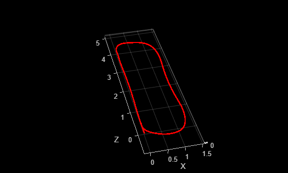
Use the monovslam class to easily invoke the entire monocular visual SLAM pipeline in just a few lines of code.

vslam = monovslam(intrinsics,MaxNumPoints=2e3,SkipMaxFrames=15,...
    TrackFeatureRange=[30,120],LoopClosureThreshold=70);

% Process each image frame 
for i = 1:numel(imds.Files)
    addFrame(vslam,readimage(imds,i));

    if hasNewKeyFrame(vslam)
        % Display 3-D map points and camera trajectory
        plot(vslam,CameraSize=0.01);
    end

    % Get current status of system
    status = checkStatus(vslam);
    
    % Stop adding frames when tracking is lost
    if status == uint8(0)
        break
    end
end

Figure contains an axes object. The axes object with xlabel X, ylabel Y contains 12 objects of type line, text, patch, scatter. This object represents Camera trajectory.

% Plot intermediate results and Wait until all images are processed
while ~isDone(vslam)
    if hasNewKeyFrame(vslam)
        plot(vslam);
    end
end

% Get final 3-D map points and camera poses
xyzPoints = mapPoints(vslam);
[camPoses,viewIds] = poses(vslam);

You can evaluate the optimized camera trajectory against the ground truth obtained from the simulation. Since the images are generated from a monocular camera, the trajectory of the camera can only be recovered up to an unknown scale factor. You can approximately compute the scale factor from the ground truth, thus simulating what you would normally obtain from an external sensor.

helperEstimateTrajectoryError(gTruth(viewIds), camPoses, useMonoCamera);

Absolute RMSE for key frame trajectory (m): 0.27744

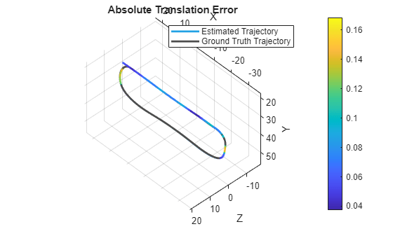
Stereo Visual SLAM Algorithm

In a monocular visual SLAM algorithm, depth cannot be accurately determined using a single camera. The scale of the map and of the estimated trajectory is unknown and drifts over time. Additionally, because map points often cannot be triangulated from the first frame, bootstrapping the system requires multiple views to produce an initial map. Using a stereo camera solves these problems and provides a more reliable visual SLAM solution. The class stereovslam implements the stereo visual SLAM pipeline.

% Select stereo camera
useMonoCamera = 0;

% Inspect the stereo camera
open_system([modelName, '/Camera/Stereo']);
snapnow;

% Set stereo camera baseline
baseline = 0.5; % In meters

% Maximum disparity in stereo images
maxDisparity = 48;

% Run simulation
simOut = sim(modelName);

Figure Video Viewer contains an axes object and other objects of type uiflowcontainer, uimenu, uitoolbar. The axes object contains an object of type image.

Figure contains an axes object. The axes object with xlabel X, ylabel Y contains 12 objects of type line, text, patch, scatter. This object represents Camera trajectory.

snapnow;

Extract Stereo Images

[imdsLeft, imdsRight] = helperGetCameraImagesStereo(simOut);

% Extract ground truth as an array of rigidtform3d objects
gTruth = helperGetSensorGroundTruth(simOut);

Run the stereo visual SLAM algorithm using the stereovslam class.

vslam = stereovslam(intrinsics,baseline,MaxNumPoints=1e3,SkipMaxFrames=20,...
    DisparityRange=[0,maxDisparity],LoopClosureThreshold=100);

for i = 1:numel(imdsLeft.Files)
    ILeft  = readimage(imdsLeft,i);
    IRight = readimage(imdsRight,i);
    addFrame(vslam,ILeft,IRight);
    
    if hasNewKeyFrame(vslam)        
        % Display 3-D map points and camera trajectory
        ax = plot(vslam);
    end
    
    % Get current status of system
    status = checkStatus(vslam);
    
    % Stop adding frames when tracking is lost
    if status == uint8(0)
        break
    end
end

% Adjust axis limits to display more 3-D map points 
set(ax, XLim=[-40, 40]);
set(ax, YLim=[-2, 10]);
set(ax, ZLim=[-10, 100]);

Figure contains an axes object. The axes object with xlabel X, ylabel Y contains 12 objects of type line, text, patch, scatter. This object represents Camera trajectory.

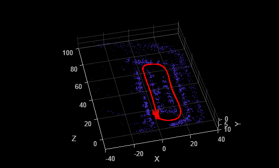
% Plot intermediate results and Wait until all images are processed
while ~isDone(vslam)
    if hasNewKeyFrame(vslam)
        plot(vslam);
    end
end

% Get final 3-D map points and camera poses
xyzPoints = mapPoints(vslam);
[camPoses,viewIds] = poses(vslam);

% Compare against the ground truth
helperEstimateTrajectoryError(gTruth(viewIds), camPoses, useMonoCamera);

Absolute RMSE for key frame trajectory (m): 0.71967

Dense Reconstruction from Stereo Images

Given the refined camera poses, you can perform dense reconstruction from the stereo images corresponding to the key frames.

pointCloudsAll = helperDenseReconstructFromStereo(imdsLeft, imdsRight, ...
    viewIds, camPoses, maxDisparity, intrinsics, baseline);

% Visualize the scene
figure(Position=[1100 600 1000 500]);
ax = pcshow(pointCloudsAll,VerticalAxis="y", VerticalAxisDir="down");
xlabel('X')
ylabel('Y')
zlabel('Z')

% Display bird's eye view of the parking lot
view(ax, [0 -1 0]);
camroll(ax, 90);

Figure contains an axes object. The axes object with xlabel X, ylabel Y contains an object of type scatter.

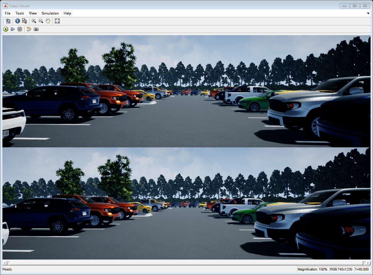
Close model and figures.

close_system(modelName, 0);

Color does not exist
CurrentAxes does not exist
UIModeEnabled does not exist
WindowButtonUpFcn does not exist
WindowButtonDownFcn does not exist
WindowKeyPressFcn does not exist
WindowKeyReleaseFcn does not exist
KeyPressFcn does not exist
KeyReleaseFcn does not exist
MenuBarMode does not exist
ToolBarMode does not exist

close all

Supporting Functions

helperGetCameraImages Get camera output

function imds = helperGetCameraImages(simOut)
% Save image data to a temporary folder
dataFolder   = fullfile(tempdir, 'parkingLotImages', filesep); 
folderExists = exist(dataFolder, 'dir');
if ~folderExists  
    mkdir(dataFolder);
end

files = dir(dataFolder);
if numel(files) < 3
    numFrames = numel(simOut.images.Time);
    for i = 3:numFrames % Ignore the first two frames
        img = squeeze(simOut.images.Data(:,:,:,i));
        imwrite(img, [dataFolder, sprintf('%04d', i-2), '.png'])
    end
end

% Create an imageDatastore object to store all the images
imds = imageDatastore(dataFolder);
end

helperGetCameraImagesStereo Get camera output

function [imdsLeft, imdsRight] = helperGetCameraImagesStereo(simOut)
% Save image data to a temporary folder
dataFolderLeft   = fullfile(tempdir, 'parkingLotStereoImages', filesep, 'left', filesep);
dataFolderRight  = fullfile(tempdir, 'parkingLotStereoImages', filesep, 'right', filesep);
folderExists     = exist(dataFolderLeft, 'dir');
if ~folderExists  
    mkdir(dataFolderLeft);
    mkdir(dataFolderRight);
end

files = dir(dataFolderLeft);
if numel(files) < 3
    numFrames = numel(simOut.imagesLeft.Time);
    for i = 3:numFrames % Ignore the first two frames
        imgLeft = squeeze(simOut.imagesLeft.Data(:,:,:,i));
        imwrite(imgLeft, [dataFolderLeft, sprintf('%04d', i-2), '.png'])
        
        imgRight = squeeze(simOut.imagesRight.Data(:,:,:,i));
        imwrite(imgRight, [dataFolderRight, sprintf('%04d', i-2), '.png'])
    end
end

% Use imageDatastore objects to store the stereo images
imdsLeft  = imageDatastore(dataFolderLeft);
imdsRight = imageDatastore(dataFolderRight);
end

helperGetSensorGroundTruth Save the sensor ground truth

function gTruth = helperGetSensorGroundTruth(simOut)
numFrames = numel(simOut.location.Time);
gTruth = repmat(rigidtform3d, numFrames-2, 1);
for i = 1:numFrames-2 % Ignore the first two frames
    gTruth(i).Translation = squeeze(simOut.location.Data(:, :, i+2));
    % Ignore the roll and the pitch rotations since the ground is flat
    yaw = double(simOut.orientation.Data(:, 3, i+2));
    gTruth(i).R = [cos(yaw), -sin(yaw), 0; ...
        sin(yaw), cos(yaw), 0; ...
        0, 0, 1];
end
end

helperEstimateTrajectoryError Calculate the tracking error

function rmse = helperEstimateTrajectoryError(gTruth, camPoses, useMonoCamera)
estimatedLoc = vertcat(camPoses.Translation);
actualLoc    = vertcat(gTruth.Translation);

if useMonoCamera
    scale = median(vecnorm(actualLoc(2:5:end,:) - actualLoc(1,:), 2, 2)./ ...
        vecnorm(estimatedLoc(2:5:end,:) - estimatedLoc(1,:), 2, 2));
    scaledLoc = estimatedLoc * scale;
    [~,~,rmse] = pcregistericp(pointCloud(estimatedLoc), pointCloud(scaledLoc));
else
    [~,~,rmse] = pcregistericp(pointCloud(estimatedLoc), pointCloud(actualLoc));
end

disp(['Absolute RMSE for key frame trajectory (m): ', num2str(rmse)]);
end

helperDenseReconstructFromStereo Perform dense reconstruction from stereo images with known camera poses

function pointCloudsAll = helperDenseReconstructFromStereo(imdsLeft, imdsRight, ...
    addedFramesIdx, optimizedPoses, maxDisparity, intrinsics, baseline)

imageSize = intrinsics.ImageSize;
ptClouds =  repmat(pointCloud(zeros(1, 3)), numel(addedFramesIdx), 1);

% Construct the reprojection matrix for 3-D reconstruction
reprojectionMatrix = [1, 0, 0, -intrinsics.PrincipalPoint(1); 
    0, 1, 0, -intrinsics.PrincipalPoint(2);
    0, 0, 0, intrinsics.FocalLength(1);
    0, 0, 1/baseline, 0];

for i = 1: numel(addedFramesIdx)
    I1 = readimage(imdsLeft,  double(addedFramesIdx(i)));
    I2 = readimage(imdsRight, double(addedFramesIdx(i)));
    disparityMap = disparitySGM(im2gray(I1), im2gray(I2), DisparityRange=[0, maxDisparity],UniquenessThreshold=20);
    xyzPoints  = reconstructScene(disparityMap, reprojectionMatrix);
    
    % Ignore the upper half of the images which mainly show the sky
    xyzPoints(1:100, :, :) = NaN;
    
    xyzPoints  = reshape(xyzPoints, [imageSize(1)*imageSize(2), 3]);

    validIndex = xyzPoints(:, 3) > 0 & xyzPoints(:, 3) < 40/reprojectionMatrix(4, 3);
    
    xyzPoints  = xyzPoints(validIndex, :);
    colors = reshape(I1, [imageSize(1)*imageSize(2), 3]);
    colors = colors(validIndex, :);

    xyzPoints  = transformPointsForward(optimizedPoses(i), xyzPoints); 
    ptCloud = pointCloud(xyzPoints, Color=colors);
    ptClouds(i) = pcdownsample(ptCloud, random=0.2); 
end

% Concatenate the point clouds
pointCloudsAll = pccat(ptClouds);
end