Reconstruct Detailed Surface Structure Using Shape from Shading

R2026b

Since R2026b

This example uses:

This example shows how to add high-frequency surface detail to stereo depth maps using Shape from Shading (SfS). SfS recovers fine geometry from image shading cues, complementing stereo methods that capture overall shape but miss small-scale features. This technique applies wherever a coarse depth estimate obtained from stereo matching, LiDAR, structured light, or depth sensors needs refinement using shading cues under known or estimated directional lighting. Starting from pre-computed camera poses created using Structure from Motion (SfM) and dense stereo depth of the asteroid Bennu, you estimate the sun direction and then solve a Poisson equation that corrects depth gradients to match observed shading. The refined depth reveals fine-scale craters and ridges that stereo matching alone cannot resolve with high accuracy.

Load Pre-Computed Data

Load depth maps, images, camera poses, and camera intrinsics for 4 views of asteroid Bennu [4]. These were pre-computed using the sfm object for Structure from Motion, followed by dense stereo matching using opticalFlowRAFT. See the Dense 3-D Reconstruction of Asteroid Surface from Image Sequence example for more information.

The data includes:

depthMaps — Per-pixel distance (in world units) from the camera center to the surface along each ray.
images — Grayscale double-precision images (intensity in [0, 1]).
poses — 3-D camera-to-world poses obtained from Structure from Motion (SfM).
intrinsics — cameraIntrinsics object encoding internal parameters of the camera such as the focal length and principal point.

load("bennuSfSData.mat","depthMaps","images","poses","intrinsics")
images = cellfun(@im2double, images, UniformOutput=false);
numViews = numel(depthMaps);

Display the four input views as a montage. Each image is a 1024-by-1024 grayscale frame captured during the OSIRIS-REx preliminary survey of asteroid Bennu [4].

figure
montage(images)
title("Input Views of Asteroid")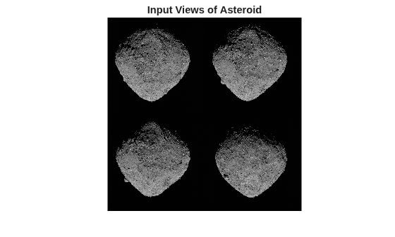

Figure contains an axes object. The hidden axes object with title Input Views of Asteroid contains an object of type image.

Visualize Input Data for Single View

Display the stereo depth map and the surface normal map side-by-side.

The helperNormalsFromDepth supporting function computes surface normals from the depth map using central differences on back-projected 3-D points. At each pixel, the function back-projects to a 3-D point, computes tangent vectors via finite differences, and takes their cross product to obtain the surface normal. The RGB channels of the normal map encode the (X, Y, Z) components of the unit normal in camera coordinates. For implementation details, see helperNormalsFromDepth.

viewIdx = 1;

normals = helperNormalsFromDepth(depthMaps{viewIdx},intrinsics);

figure
tiledlayout(1,2)

nexttile
imagesc(depthMaps{viewIdx})
axis image
colorbar
title("Depth Map (View 1)")

nexttile
% Map unit normals in [-1,1] to [0,1] for display
imshow( (normals + 1)/2 )  
title("Surface Normal Map (View 1)")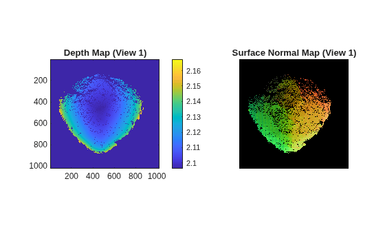

Figure contains 2 axes objects. Axes object 1 with title Depth Map (View 1) contains an object of type image. Hidden axes object 2 with title Surface Normal Map (View 1) contains an object of type image.

Observe that the depth map shows smooth, low-frequency surface shape recovered by stereo, but lacks the fine detail visible in the intensity images. The normal map highlights subtle orientation changes that SfS exploits to recover high-frequency geometry.

Estimate Direction of Illumination

Under a Lambertian reflectance model [1], observed image intensity $I$ at a surface point satisfies: $I = ρ \cdot (n \cdot l)$ , where

$ρ$ is the surface albedo (fraction of incident light reflected by the surface).
$n$ is the outward unit surface normal direction.
$l$ is the unit vector pointing toward the light source, the Sun.
$n \cdot l$ is the cosine of the angle between the surface normal and the light direction.

This model assumes that the Sun is infinitely far away, resulting in parallel rays illuminating the asteroid surface. It also assumes a diffuse surface, reflecting incident light equally in all directions. Both assumptions hold here: the Sun-Bennu distance is significantly larger than the asteroid diameter, and Bennu's rough surface exhibits approximately diffuse reflectance.

To estimate the light direction, stack surface normals ( $N$ ) and intensities ( $I$ ) from all views and solve the resulting linear system: $N s = I$ where $s = ρ \cdot l$ . The least-squares solution to this system gives the scaled light direction $s$ . Normalizing $s$ yields $l$ , which is the unit vector in the estimated light direction.

allNormals = cell(numViews,1);
allIntensities = cell(numViews,1);

for i = 1:numViews
    normalsCam = helperNormalsFromDepth(depthMaps{i},intrinsics);

    % Rotate normals from camera frame to world frame using the camera
    % orientation from SfM. This aligns all views so they share a common
    % light direction vector.
    R = poses{i}.R;
    [H,W,~] = size(normalsCam);
    n = reshape(normalsCam,[],3) * R';
    normalsWorld = reshape(n,H,W,3);

    % Select pixels with valid depth, moderate intensity (avoiding
    % saturated highlights and deep shadows), and valid normals.
    valid = ~isnan(depthMaps{i}) & images{i} > 0.1 & images{i} < 0.9 ...
        & ~isnan(normalsWorld(:,:,1));
    idx = find(valid);
    nx = normalsWorld(:,:,1);
    ny = normalsWorld(:,:,2);
    nz = normalsWorld(:,:,3);
    N = [nx(idx) ny(idx) nz(idx)];
    I = images{i}(idx);

    allNormals{i} = N;
    allIntensities{i} = I;
end

% Concatenate into numeric arrays for the least-squares solver                                                     
allNormals = vertcat(allNormals{:});                                                                          
allIntensities = vertcat(allIntensities{:});

Solve the linear system using the backslash operator, which provides the least-squares solution to the system.

s = allNormals \ allIntensities;
lightDir = s'/norm(s)

lightDir = 1×3

    -0.0205    0.8435    -0.5368

The estimated light direction is a 3-D unit vector in world coordinates. It is consistent across all views because we transformed normals into the common world frame before solving.

Estimate Depth Gradients from Lambertian Shading Model

Compute shading-derived depth gradients for one view.

Estimate Surface Normal Using Reflectance Model

Invert the Lambertian reflectance equation $I = ρ \cdot (n \cdot l)$ to determine the orientation of each surface normal with respect to the light source that produces the observed intensity at that pixel [1]. A bright pixel faces the Sun nearly head-on, while a dark pixel more likely belongs to a surface oriented away from the direction of illumination.

viewIdx = 1;                                                                          
Z = depthMaps{viewIdx};
I = images{viewIdx};
fx = intrinsics.FocalLength(1);
fy = intrinsics.FocalLength(2);

% Light direction in camera frame
lightDirCam = lightDir * poses{viewIdx}.R;
L = reshape(lightDirCam, 1, 1, 3); % reshaped to 1x1x3 for array operations

% Normals from coarse stereo depth
normals = helperNormalsFromDepth(Z, intrinsics);

nDotLStereo = sum(normals .* L, 3);
validMask = ~isnan(Z) & I > 0.02;

% Estimate albedo
rho = mean(I(validMask) ./ max(nDotLStereo(validMask), 0.05), "omitnan");

% Expected n·l from observed intensity by inverting Lambertian model
nDotLShading = min(I / max(rho,eps), 1);

% Adjust existing stereo-derived normals along the light direction to match the observed shading.
normalsRefined = nDotLShading .* L + (normals - nDotLStereo .* L);

% Clip low-magnitude vectors and normalize to unit length.
mag = vecnorm(normalsRefined, 2, 3);
mag(mag < eps) = 1;
normalsRefined = normalsRefined ./ mag;

Estimate Depth Gradients Using Normals and Camera Geometry

Convert each normal to local depth map gradients using pinhole camera geometry and known values of camera intrinsics parameters [2,6]. For a pinhole camera, the relationship between surface normal $(n_{x}, n_{y}, n_{z})$ and depth slopes $(p, q)$ is: $p = - \frac{Z . n_{x}}{f_{x} . n_{z}}$ , $q = - \frac{Z . n_{y}}{f_{y} . n_{z}}$ .

% Clamp z-component of normals (nz) away from zero since it is in the denominator
nz = normalsRefined(:,:,3);
nz(abs(nz) < 0.1) = sign(nz(abs(nz) < 0.1) + eps) * 0.1;

% Derived depth slopes using known camera intrinsics
p = -Z .* normalsRefined(:,:,1) ./ (fx * nz);
q = -Z .* normalsRefined(:,:,2) ./ (fy * nz);

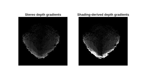
Visualize the depth gradient field derived from shading. Compare it with the depth gradients of the original coarse depth map from stereo. The shading-derived depth gradient field has higher magnitude and reveals finer details compared to the stereo depth map gradients. The next section uses this gradient field to refine the stereo depth.

dZdx = (Z(:,[2:end end]) - Z(:,[1 1:end-1])) / 2;
dZdy = (Z([2:end end],:) - Z([1 1:end-1],:)) / 2;
magStereo = sqrt(dZdx.^2 + dZdy.^2);
magShading = sqrt(p.^2 + q.^2);

figure                                                                               
tiledlayout(1,2,TileSpacing="compact")
cRange = [0 max(magShading(:),[],"omitnan")*0.8];
nexttile
imagesc(magStereo, cRange);
axis image off;
title("Stereo depth gradients")                                
nexttile
imagesc(magShading, cRange);
axis image off;
title("Shading-derived depth gradients")
colormap(gray)

Figure contains 2 axes objects. Hidden axes object 1 with title Stereo depth gradients contains an object of type image. Hidden axes object 2 with title Shading-derived depth gradients contains an object of type image.

Refine Depth Maps with Shape from Shading

For each view, transform the estimated Sun direction from world coordinates into the camera frame, then solve a screened Poisson equation to refine the depth. The screened Poisson equation [5] is a partial differential equation of the form: $(λ I - Δ) Z = λ Z_{0} + \nabla \cdot g$ .

$Z_{0}$ is the original stereo depth which serves as a coarse initialization point for the optimization.
$Z$ is the refined depth that is iteratively estimated and refined.
$Δ$ is the discrete Laplacian of the depth map $Z$ , which captures the local curvature of the surface defined by the depth map.
$g$ is the shading-derived gradient field of the depth map described in the previous section.

This formulation was introduced by Nehab et al. [3] to fuse position and normal information for surface reconstruction, balancing two objectives:

Shading fidelity: depth gradients should produce normals whose dot product with the light direction matches observed intensity.
Stereo prior: the refined depth should not drift far from the original stereo estimate (controlled by the parameter $λ$ ).

depthMapsRefined = cell(numViews,1);

for i = 1:numViews
    % Transform the estimated sun direction from the world coordinate 
    % frame into the camera coordinate frame for the i-th view
    lightDirCam = lightDir * poses{i}.R;

    fprintf("Processing view %d/%d\n",i,numViews)

    depthMapsRefined{i} = helperRefineDepthSfS( ...
        depthMaps{i},images{i},intrinsics,lightDirCam);
end

Processing view 1/4
Processing view 2/4
Processing view 3/4
Processing view 4/4

Reconstruct 3-D Point Clouds

Back-project both the original stereo and the SfS-refined depth maps into world coordinates to build colored point clouds. Subsample pixels with a stride of 2 and apply a border offset of 50 pixels to avoid edge artifacts. Transform each local camera-frame point cloud into the world frame using the corresponding camera pose.

offset = 50;
depthRange = [0 5];
depthScaleFactor = 1;
[X,Y] = meshgrid(offset:2:intrinsics.ImageSize(2)-offset, ...
    offset:2:intrinsics.ImageSize(1)-offset);
pts = [X(:) Y(:)];

[H,W] = size(images{1});                                                                                     
linearIdx = sub2ind([H W], Y(:), X(:)); 

ptCloudsStereo = cell(numViews,1);
ptCloudsSfS = cell(numViews,1);

for i = 1:numViews

    fprintf("Processing view %d/%d\n",i,numViews)

    % Convert grayscale to RGB for natural 3-channel color indexing                                          
    imgRGB = repmat(images{i}, 1, 1, 3);                                                                
    imgFlat = reshape(imgRGB, [], 3);
    colors = imgFlat(linearIdx,:);

    % Stereo point cloud
    pc = pcfromdepth(depthMaps{i},depthScaleFactor,intrinsics,...
        ImagePoints=pts,DepthRange=depthRange);
    validIdx = find(~isnan(pc.Location(:,1)));
    xyz = transformPointsForward(poses{i},pc.Location(validIdx,:));
    ptCloudsStereo{i} = pointCloud(xyz,Color=colors(validIdx,:));

    % Shape-from-Shading-refined point cloud
    pc = pcfromdepth(depthMapsRefined{i},depthScaleFactor,intrinsics,...
        ImagePoints=pts,DepthRange=depthRange);
    validIdx = find(~isnan(pc.Location(:,1)));
    xyz = transformPointsForward(poses{i},pc.Location(validIdx,:));
    ptCloudsSfS{i} = pointCloud(xyz,Color=colors(validIdx,:));
end

Processing view 1/4
Processing view 2/4
Processing view 3/4
Processing view 4/4

pcStereo = pccat(cat(1,ptCloudsStereo{:}));
pcSfS = pccat(cat(1,ptCloudsSfS{:}));

Use pcdenoise to remove outliers from the reconstructed point clouds.

pcStereo = pcdenoise(pcStereo);
pcSfS = pcdenoise(pcSfS);

Visualize 3-D Stereo Reconstruction and Lighting Direction

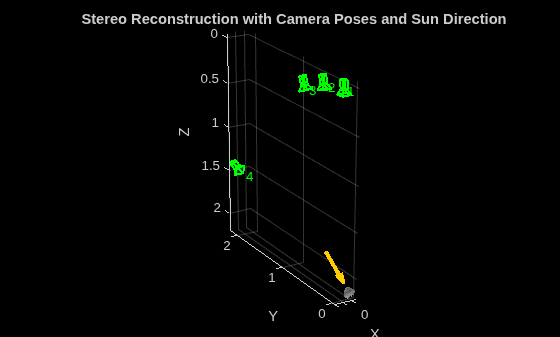
Display the stereo point cloud with the reconstructed camera positions and the estimated Sun direction vector. The yellow arrow indicates the direction sunlight arrives from.

figure

% Downsample point cloud for faster interactive visualization
pcStereoVis = pcdownsample(pcStereo, "gridAverage", 0.005);
pcshow(pcStereoVis,MarkerSize=5);

% Display the cameras
hold on
camPoses = arrayfun(@(i) poses{i},1:numViews);
plotCamera(camPoses,Color="green",Size=0.05,Opacity=0.1)

% Display the Sun direction as an arrow pointing from the light source
center = mean(pcStereo.Location,1);
sunStart = center + 0.5*lightDir;
quiver3(sunStart(1),sunStart(2),sunStart(3), ...
    -lightDir(1),-lightDir(2),-lightDir(3),0.4, ...
    Color=[1 0.8 0],LineWidth=3,MaxHeadSize=1.0)

% Axis conventions and viewing direction
set(gca,"ZDir","reverse")
view(-30, 20)

hold off
axis equal
xlabel("X")
ylabel("Y")
zlabel("Z")
title("Stereo Reconstruction with Camera Poses and Sun Direction")

Reconstruct 3-D Surface Geometry from Point Cloud

Downsample the point clouds to reduce the runtime for Poisson surface reconstruction. Set the grid size to 0.3% of the point cloud's spatial extent, balancing meshing speed against preserving fine surface detail.

gridSizePct = 0.3;
extents = [diff(pcStereo.XLimits), diff(pcStereo.YLimits), diff(pcStereo.ZLimits)];
gridSize = norm(extents) * gridSizePct / 100;
pcStereoDS = pcdownsample(pcStereo,"gridAverage",gridSize);
pcSfSDS = pcdownsample(pcSfS,"gridAverage",gridSize);

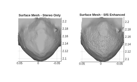
Reconstruct surface meshes from the point clouds of stereo and shading using Poisson surface reconstruction. This is a computationally intensive step and can take 30-60 seconds on a typical desktop computer.

meshStereo = pc2surfacemesh(pcStereoDS,"poisson");
meshSfS = pc2surfacemesh(pcSfSDS,"poisson");

Compare Reconstructed 3-D Surface Geometry

Render the two surfaces side-by-side for visual comparison. The lighting and material texture settings in the visualization highlight fine-grained differences in the reconstructed surfaces. The SfS-enhanced mesh reveals craters, ridges, and boulder features that are absent from the stereo-only reconstruction.

figure
tiledlayout(1,2)

nexttile
trisurf(meshStereo.Faces, ...
    meshStereo.Vertices(:,1),meshStereo.Vertices(:,2),meshStereo.Vertices(:,3), ...
    FaceColor=[0.7 0.7 0.7],EdgeColor="none")
axis equal
view(180,0)
lighting gouraud
camlight headlight
material dull
title("Surface Mesh - Stereo Only")

nexttile
trisurf(meshSfS.Faces, ...
    meshSfS.Vertices(:,1),meshSfS.Vertices(:,2),meshSfS.Vertices(:,3), ...
    FaceColor=[0.7 0.7 0.7],EdgeColor="none")
axis equal
view(180,0)
lighting gouraud
camlight headlight
material dull
title("Surface Mesh - SfS Enhanced")

Figure contains 2 axes objects. Axes object 1 with title Surface Mesh - Stereo Only contains an object of type patch. Axes object 2 with title Surface Mesh - SfS Enhanced contains an object of type patch.

Supporting Functions

`helperNormalsFromDepth`

function normals = helperNormalsFromDepth(depthMap,intrinsics)
% Compute surface normals from a depth map using central
% differences on the back-projected 3D points.

[H,W] = size(depthMap);
fx = intrinsics.FocalLength(1);
fy = intrinsics.FocalLength(2);
cx = intrinsics.PrincipalPoint(1);
cy = intrinsics.PrincipalPoint(2);

[u,v] = meshgrid(1:W,1:H);
X = (u - cx) .* depthMap / fx;
Y = (v - cy) .* depthMap / fy;
Z = depthMap;

% Central differences for tangent vectors
dXdu = zeros(H,W); dYdu = zeros(H,W); dZdu = zeros(H,W);
dXdv = zeros(H,W); dYdv = zeros(H,W); dZdv = zeros(H,W);

dXdu(:,2:end-1) = (X(:,3:end) - X(:,1:end-2))/2;
dYdu(:,2:end-1) = (Y(:,3:end) - Y(:,1:end-2))/2;
dZdu(:,2:end-1) = (Z(:,3:end) - Z(:,1:end-2))/2;

dXdv(2:end-1,:) = (X(3:end,:) - X(1:end-2,:))/2;
dYdv(2:end-1,:) = (Y(3:end,:) - Y(1:end-2,:))/2;
dZdv(2:end-1,:) = (Z(3:end,:) - Z(1:end-2,:))/2;

% Cross product of the tangent vectors gives normals
nx = dYdu.*dZdv - dZdu.*dYdv;
ny = dZdu.*dXdv - dXdu.*dZdv;
nz = dXdu.*dYdv - dYdu.*dXdv;

% Validity checks and filters
mag = sqrt(nx.^2 + ny.^2 + nz.^2);
mag(mag < eps) = nan;
normals = cat(3,nx./mag,ny./mag,nz./mag);

% Ensure normals point toward camera (nz < 0)
flip = normals(:,:,3) > 0;
normals(:,:,1) = normals(:,:,1) .* (1 - 2*flip);
normals(:,:,2) = normals(:,:,2) .* (1 - 2*flip);
normals(:,:,3) = normals(:,:,3) .* (1 - 2*flip);
end

`helperRefineDepthSfS`

function depthRefined = helperRefineDepthSfS(depthMap,I,intrinsics,lightDirCam)
% Refine a stereo depth map using Shape from Shading.
% Solves a screened Poisson equation whose target gradients come from the
% shading constraints.

lambdaDepth = 0.02;       % Regularization weight (higher = closer to stereo)
numIterations = 5;        % Max number of solver iterations
minNdotL = 0.05;          % Clamp to avoid division by zero in shadows
relativeTolerance = 1e-6; % Exit if objective function changes less than this value

[H,W] = size(depthMap);
fx = intrinsics.FocalLength(1);
fy = intrinsics.FocalLength(2);
lx = lightDirCam(1); ly = lightDirCam(2); lz = lightDirCam(3);

validMask = ~isnan(depthMap) & I > 0.02;
validIdx = find(validMask);
numValid = numel(validIdx);

if numValid < 100
    fprintf("skipped (%d valid pixels)\n",numValid)
    depthRefined = depthMap;
    return
end

% Build 4-connected neighbor graph
pixelIndex = zeros(H,W);
pixelIndex(validIdx) = 1:numValid;
[rows,cols] = ind2sub([H W],validIdx);

hasL = cols > 1 & validMask(sub2ind([H W],rows,max(cols-1,1)));
idxL = sub2ind([H W],rows(hasL),cols(hasL)-1);
hasR = cols < W & validMask(sub2ind([H W],rows,min(cols+1,W)));
idxR = sub2ind([H W],rows(hasR),cols(hasR)+1);
hasU = rows > 1 & validMask(sub2ind([H W],max(rows-1,1),cols));
idxU = sub2ind([H W],rows(hasU)-1,cols(hasU));
hasD = rows < H & validMask(sub2ind([H W],min(rows+1,H),cols));
idxD = sub2ind([H W],rows(hasD)+1,cols(hasD));

% Build and factorize A = λI + L (constant across iterations)
numNbrs = double(hasL) + double(hasR) + double(hasU) + double(hasD);
offI = [find(hasL); find(hasR); find(hasU); find(hasD)];
offJ = [pixelIndex(idxL); pixelIndex(idxR); pixelIndex(idxU); pixelIndex(idxD)];
offV = -ones(numel(offI),1);
diagV = lambdaDepth + numNbrs;
A = sparse([(1:numValid)'; double(offI)], ...
[(1:numValid)'; double(offJ)],[diagV; offV],numValid,numValid);
dA = decomposition(A,"chol");

% Initialize depth
Z = depthMap;
Z(~validMask) = 0;
Z_stereo = Z;

% Initial scalar albedo
normals_cam = helperNormalsFromDepth(depthMap,intrinsics);
ndotl = normals_cam(:,:,1)*lx + normals_cam(:,:,2)*ly + normals_cam(:,:,3)*lz;
ndotl = max(ndotl,minNdotL);
rho = mean(I(validIdx) ./ ndotl(validIdx),"omitnan");

prevMSE = inf;
for iter = 1:numIterations
    Z_prev = Z;

    % Compute normals from current depth estimate
    Zn = Z; Zn(~validMask) = NaN;
    normals_cam = helperNormalsFromDepth(Zn,intrinsics);
    nx = normals_cam(:,:,1);
    ny = normals_cam(:,:,2);
    nz = normals_cam(:,:,3);
    
    % Target n·l from shading: intensity I = rho*(n·l)
    target_ndotl = min(max(I/max(rho,eps),0),1);
    
    % Correct normals: replace light-parallel component with target
    ndotl_cur = nx*lx + ny*ly + nz*lz;
    n_new_x = target_ndotl*lx + (nx - ndotl_cur*lx);
    n_new_y = target_ndotl*ly + (ny - ndotl_cur*ly);
    n_new_z = target_ndotl*lz + (nz - ndotl_cur*lz);
    mag = sqrt(n_new_x.^2 + n_new_y.^2 + n_new_z.^2);
    mag(mag < eps) = 1;
    n_new_x = n_new_x./mag;
    n_new_y = n_new_y./mag;
    n_new_z = n_new_z./mag;
    
    % Convert corrected normals to depth gradients (perspective model)
    nz_safe = n_new_z;
    nz_safe(abs(nz_safe) < 0.1) = sign(nz_safe(abs(nz_safe) < 0.1)+eps)*0.1;
    p = -Z .* n_new_x ./ (fx*nz_safe);
    q = -Z .* n_new_y ./ (fy*nz_safe);
    p(~validMask | isnan(p)) = 0;
    q(~validMask | isnan(q)) = 0;
    
    % Smooth gradients (3x3 box filter)
    kernel = ones(3)/9;
    wt = conv2(double(validMask),kernel,"same");
    p = conv2(p.*validMask,kernel,"same") ./ max(wt,eps);
    q = conv2(q.*validMask,kernel,"same") ./ max(wt,eps);
    p(~validMask | isnan(p)) = 0;
    q(~validMask | isnan(q)) = 0;
    
    % Divergence (graph-consistent with Laplacian)
    divTarget = zeros(numValid,1);
    ri = find(hasR);
    divTarget(ri) = divTarget(ri) - p(validIdx(ri));
    li = find(hasL);
    divTarget(li) = divTarget(li) + p(idxL);
    di = find(hasD);
    divTarget(di) = divTarget(di) - q(validIdx(di));
    ui = find(hasU);
    divTarget(ui) = divTarget(ui) + q(idxU);
    
    % Solve screened Poisson: (λI + L)Z = λ*Z_stereo + div(g)
    rhs = lambdaDepth*Z_stereo(validIdx) + divTarget;
    Z(validIdx) = dA \ rhs;
    
    % Update albedo
    Zn = Z; Zn(~validMask) = NaN;
    normals_cam = helperNormalsFromDepth(Zn,intrinsics);
    ndotl = normals_cam(:,:,1)*lx + normals_cam(:,:,2)*ly + normals_cam(:,:,3)*lz;
    ndotl = max(ndotl,minNdotL);
    rho = mean(I(validIdx) ./ ndotl(validIdx),"omitnan");
    
    % Check convergence
    currentMSE = mean((rho*ndotl(validIdx) - I(validIdx)).^2);
    stepChange = max(abs(Z(validIdx) - Z_prev(validIdx)));
    
    if stepChange < relativeTolerance
        break
    end

    % Exit the optimization if the error increases compared to previous
    % iteration.
    if iter > 1 && currentMSE > prevMSE
        Z = Z_prev;
        break
    end

    prevMSE = currentMSE;
end
depthRefined = nan(H,W);
depthRefined(validIdx) = Z(validIdx);
end

References

[1] Horn, B.K.P. "Shape from Shading: A Method for Obtaining the Shape of a Smooth Opaque Object from One View." MIT AI Memo 232, 1970.

[2] Frankot, R.T. and Chellappa, R. "A Method for Enforcing Integrability in Shape from Shading Algorithms." IEEE TPAMI, 1988.

[3] Nehab, D., Rusinkiewicz, S., Davis, J., and Ramamoorthi, R. "Efficiently Combining Positions and Normals for Precise 3D Geometry." ACM SIGGRAPH, 2005.

[4] OSIRIS-REx Camera Suite (OCAMS) Bundle https://arcnav.psi.edu/urn:nasa:pds:orex.ocams

[5] Kazhdan, M. and Hoppe, H. "Screened Poisson Surface Reconstruction." ACM Transactions on Graphics 32(3), Article 29, 2013.

[6] Horn, B.K.P. and Brooks, M.J. "The Variational Approach to Shape from Shading." Computer Vision, Graphics and Image Processing, 33(2), 174–208, 1986.