Orthogonal and Biorthogonal Filter Banks

Orthogonal Wavelet Filters

Obtain the lowpass (scaling) and highpass (wavelet) analysis and synthesis filters of wavelet.

[gtilde,htilde,g,h] = wfilters("db2");

The analysis and synthesis filters for the "db2" wavelet are just time reverses of each other. This is the case with all orthogonal wavelet filter banks. You can see this by comparing the following.

scalingFilters = [flip(gtilde); g]

scalingFilters = 2×4

    0.4830    0.8365    0.2241   -0.1294
    0.4830    0.8365    0.2241   -0.1294

waveletFilters = [flip(htilde); h]

waveletFilters = 2×4

   -0.1294   -0.2241    0.8365   -0.4830
   -0.1294   -0.2241    0.8365   -0.4830

Implement Single-Level Two-Channel Filter Bank Using dwt

Obtain the level-one DWT of the ECG signal. This is equivalent to the analysis branch (with downsampling) of the two-channel filter bank in the figure at the start of this example.

[lowpass,highpass] = dwt(wecg,gtilde,htilde);

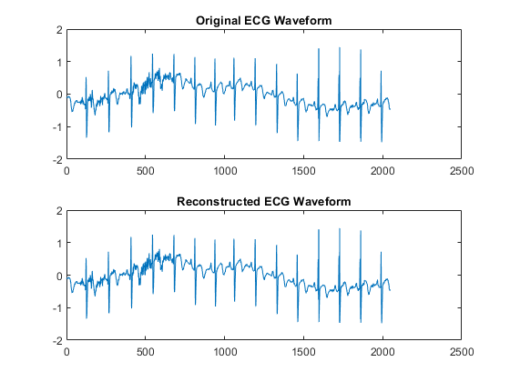
Upsample and interpolate the lowpass (scaling coefficients) and highpass (wavelet coefficients) subbands with the synthesis filters and demonstrate perfect reconstruction.

xrec = idwt(lowpass,highpass,g,h);
max(abs(wecg-xrec))

ans = 
1.3658e-12

tiledlayout(2,1)
nexttile
plot(wecg)
axis tight
title("Original ECG Waveform")
nexttile
plot(xrec)
axis tight
title("Reconstructed ECG Waveform")

Instead of providing dwt with the filters in the previous example, use the string "db2" instead. Using the wavelet family short name, "db", and filter number, 2, you do not have to specify the analysis and synthesis filters.

[lowpass,highpass] = dwt(wecg,"db2");
xrec = idwt(lowpass,highpass,"db2");

The filter number in the Daubechies's extremal phase and least asymmetric phase wavelets ("db" and "sym") refers to the number of vanishing moments. Basically, a wavelet with N vanishing moments removes a polynomial of order N-1 in the wavelet coefficients. To illustrate this, construct a signal which consists of a linear trend with additive noise.

figure
n = (0:511)/512;
x = 2*n+0.2*randn(size(n));
plot(n,x)

A linear trend is a polynomial of degree 1. Therefore, a wavelet with two vanishing moments removes this polynomial. The linear trend is preserved in the scaling coefficients and the wavelet coefficients can be regarded as consisting of only noise. Obtain the level-one DWT of the signal with the "db2" wavelet (two vanishing moments) and plot the coefficients.

[A,D] = dwt(x,'db2');
figure
tiledlayout(2,1)
nexttile
plot(A)
axis tight
title("Scaling Coefficients")
nexttile
plot(D)
axis tight
title("Wavelet Coefficients")

Implement Multilevel Two-Channel Filter Bank Using wavedec

You can use dwt and idwt to implement a two-channel orthogonal filter bank, but it is often more convenient to implement a multi-level two-channel filter bank using wavedec. The multi-level DWT iterates on the output of the lowpass (scaling) filter. In other words, the input to the second level of the filter bank is the output of the lowpass filter at level 1. A two-level wavelet filter bank is illustrated in this figure.

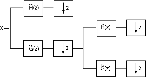
At each successive level, the number of scaling and wavelet coefficients is downsampled by two so the total number of coefficients are preserved. Obtain the level three DWT of the ECG signal using the "sym4" orthogonal filter bank.

[C,L] = wavedec(wecg,3,"sym4");

The number of coefficients by level is contained in the vector, L. The first element of L is 256, which represents the number of scaling coefficients at level 3 (the final level). The second element of L is the number of wavelet coefficients at level 3. Subsequent elements give the number of wavelet coefficients at higher levels until you reach the final element of L. The final element of L is equal to the number of samples in the original signal. The scaling and wavelet coefficients are stored in the vector C in the same order. To extract the scaling or wavelet coefficients, use appcoef or detcoef. Extract all the wavelet coefficients in a cell array and final-level scaling coefficients.

wavcoefs = detcoef(C,L,"dcells");
a3 = appcoef(C,L,"sym4");

You can plot the wavelet and scaling coefficients at their approximate positions.

cfsmatrix = zeros(numel(wecg),4);
cfsmatrix(1:2:end,1) = wavcoefs{1};
cfsmatrix(1:4:end,2) = wavcoefs{2};
cfsmatrix(1:8:end,3) = wavcoefs{3};
cfsmatrix(1:8:end,4) = a3;
figure
tiledlayout(5,1)
nexttile
plot(wecg)
title("Original Signal")
axis tight
for kk = 2:4
    nexttile
    stem(cfsmatrix(:,kk-1), ...
        marker="none",ShowBaseLine="off")
    ylabel("D"+num2str(kk-1))
    axis tight
end
nexttile
stem(cfsmatrix(:,end), ...
    marker="none", ...
    ShowBaseLine="off")
ylabel("A3")
xlabel("Sample")
axis tight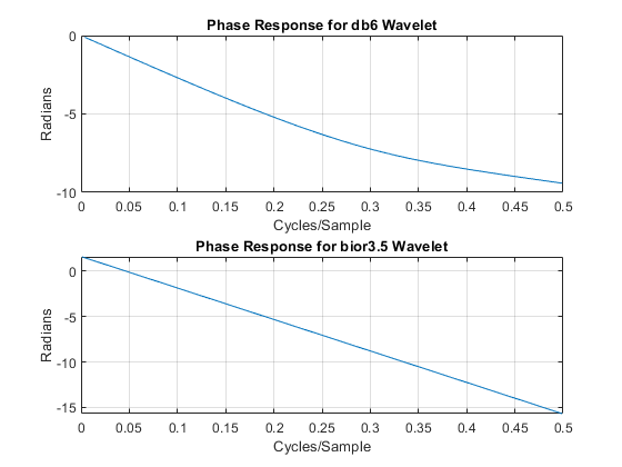

Because the critically sampled wavelet filter bank downsamples the data at each level, the analysis must stop when you have only one coefficient left. In the case of the ECG signal with 2048 samples, this must occur when $$L={\log }_{2}2048$$.

[C,L] = wavedec(wecg,log2(numel(wecg)),"sym4");
fprintf("The number of coefficients at the final level is %d. \n",L(1));

The number of coefficients at the final level is 1. 

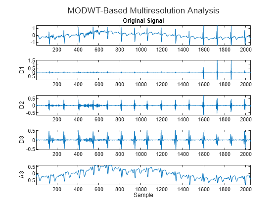
If you wish to implement an orthogonal wavelet filter bank without downsampling, you can use modwt.

ecgmodwt = modwt(wecg,"sym4",3);
ecgmra = modwtmra(ecgmodwt,"sym4");
figure
t=tiledlayout(5,1);
nexttile
plot(wecg)
axis tight
title("Original Signal")
for kk = 2:4
    nexttile
    plot(ecgmra(kk-1,:))
    axis tight
    ylabel("D"+num2str(kk-1))
end
nexttile
plot(ecgmra(end,:))
axis tight
ylabel("A3")
xlabel("Sample")
title(t,"MODWT-Based Multiresolution Analysis")

Biorthogonal Wavelet Filters

In a biorthogonal filter bank, the synthesis filters are not simply time-reversed versions of the analysis filters. The family of biorthogonal spline wavelet filters are an example of such filter banks.

[LoD,HiD,LoR,HiR] = wfilters("bior3.5");

If you examine the analysis filters (LoD, HiD) and the synthesis filters (LoR, HiR), you see that they are very different. These filter banks still provide perfect reconstruction.

[A,D] = dwt(wecg,LoD,HiD);
xrec = idwt(A,D,LoR,HiR);
max(abs(wecg-xrec))

ans = 
4.4409e-16

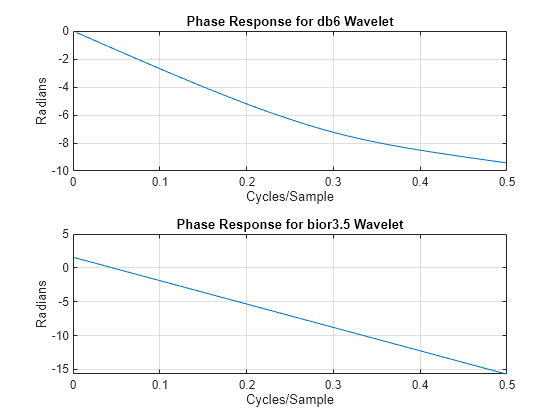
Biorthogonal filters are useful when linear phase is a requirement for your filter bank. Orthogonal filters cannot have linear phase with the exception of the Haar wavelet filter. If you have Signal Processing Toolbox™, you can look at the phase responses for an orthogonal and biorthogonal pair of wavelet filters.

[Lodb6,Hidb6] = wfilters("db6");
[PHIdb6,W] = phasez(Hidb6,1,512);
PHIbior35 = phasez(HiD,1,512);
figure
tiledlayout(2,1)
nexttile
plot(W./(2*pi),PHIdb6)
title("Phase Response for db6 Wavelet")
grid on
xlabel("Cycles/Sample")
ylabel("Radians")
nexttile
plot(W./(2*pi),PHIbior35)
title("Phase Response for bior3.5 Wavelet")
grid on
xlabel("Cycles/Sample")
ylabel("Radians")

Set the padding mode back to the original setting.

dwtmode(origmodestatus,"nodisplay")