Visualize and Recreate EWT Decomposition

Visualize EWT

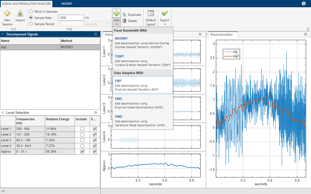
Open Signal Multiresolution Analyzer and click Import. Select sig and click Import. By default, a four-level MODWTMRA decomposition appears in the MODWT tab. In the Signal Multiresolution Analyzer tab, set the sample rate to 1000 Hz.

To generate an MRA decomposition using the empirical wavelet transform (EWT), go to the Signal Multiresolution Analyzer tab. Click Add ▼ and select EWT.

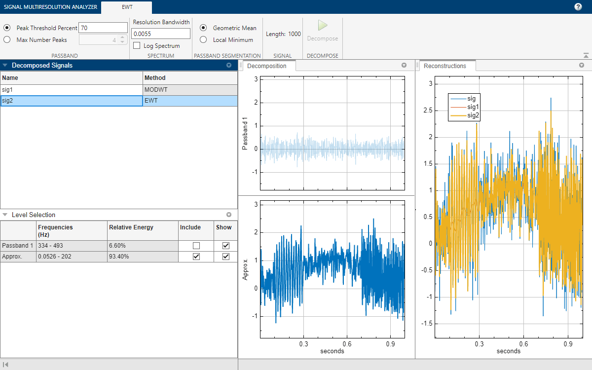
After a few moments, the EWT decomposition sig2 appears in the EWT tab. The app obtains the decomposition using the ewt function with default settings. The Level Selection pane shows the relative energies of the signal across the passbands, as well as the measured frequency ranges. With the toolstrip, you can change the EWT parameters to generate a different decomposition. You can:

Changing a value enables the Decompose button. To learn more about the parameters, see ewt and Empirical Wavelet Transform.

Change Peak Identification Method

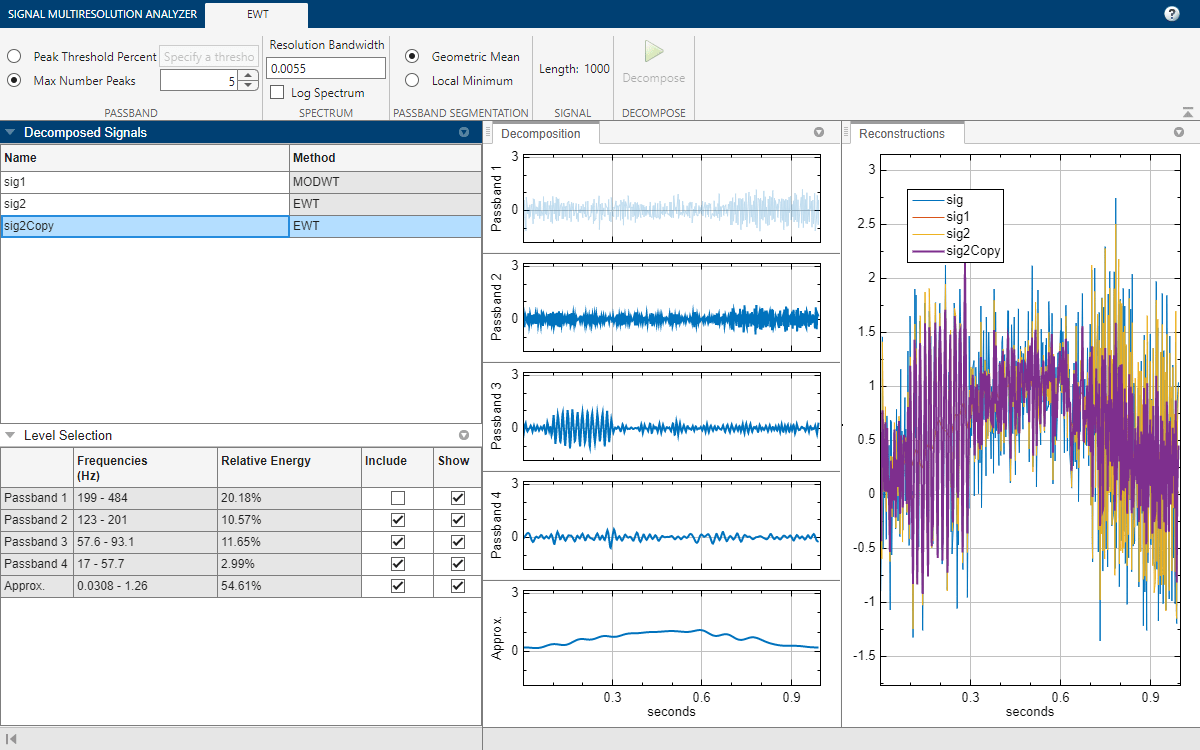
By default, the ewt function uses a threshold to determine which peaks to retain in the multitaper power spectrum of the signal. In the case of sig, ewt found two passbands. You can also choose the N largest peaks. To compare the two methods, select sig2, and on the Signal Multiresolution Analyzer tab, click Duplicate. A duplicate, sig2Copy, appears. In the EWT tab, set the value of Max Number Peaks to 5 and click Decompose. The result is a decomposition with five passbands.

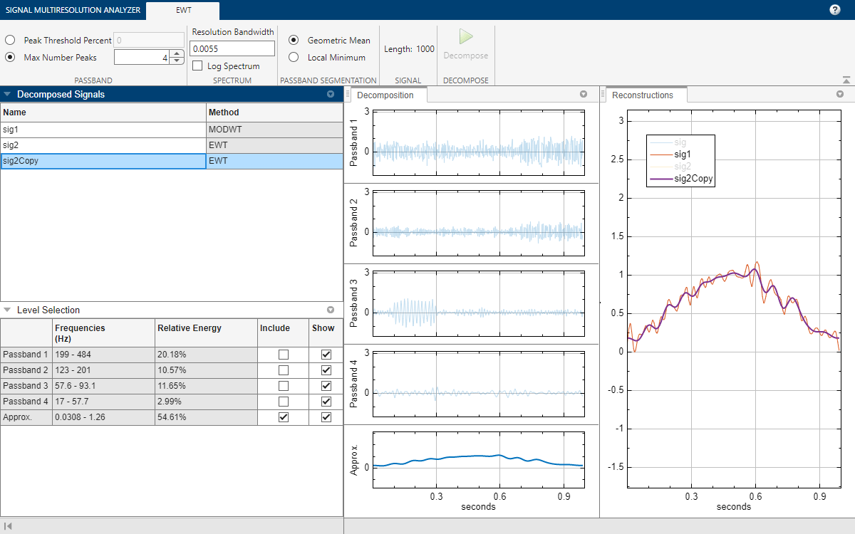
You can compare the sig2Copy approximation with the sig1 approximation by first removing passbands 2 through 4 from the sig2Copy reconstruction, and then clicking sig and sig2 in the legend in the Reconstructions pane. To remove a passband from the reconstruction, you can either clear the corresponding Include box in the Level Selection pane or click on the plot of the passband in the Decomposition pane.

Export Script

To recreate the decomposition in your workspace, in the Signal Multiresolution Analyzer tab click Export > Generate MATLAB Script. An untitled script opens in your editor with the following executable code. The true-false values in levelForReconstruction correspond to the Include boxes you selected in the Level Selection pane. You can save the script as is or modify it to apply the same decomposition settings to other signals. Run the code.

% Logical array for selecting reconstruction elements
levelForReconstruction = [false,false,false,false,true];

% Perform the decomposition using ewt
[mra,cfs,wfb,info] = ewt(sig, ...
    MaxNumPeaks=5, ...
    SegmentMethod='geomean', ...
    FrequencyResolution=0.0055, ...
    LogSpectrum=false);

% Sum down the rows of the selected multiresolution signals
sig2Copy = sum(mra(:,levelForReconstruction),2);

The columns in the MRA matrix mra correspond to the passbands and approximation in the Level Selection pane. Plot the passbands, and confirm they are identical with those in the app.

numplots = size(mra,2);
figure
for k=1:numplots
    subplot(numplots,1,k)
    plot(mra(:,k))
    if k~=numplots
        title(["Passband "+num2str(k)])
    else
        title("Approx.")
    end
    axis tight
end