Main Content

ewt

Empirical wavelet transform

Since R2020b

    Description

    mra = ewt(x) returns the multiresolution analysis (MRA) components corresponding to the empirical wavelet transform (EWT) of x. Use ewt to decompose signals using an adaptable wavelet subdivision scheme that automatically determines the empirical wavelet and scaling filters and preserves energy.

    By default, the number of empirical wavelet filters is automatically determined by identifying peaks in a multitaper power spectral estimate of x.

    example

    [mra,cfs] = ewt(x) returns the EWT analysis coefficients of x.

    [mra,cfs,wfb] = ewt(x) returns the empirical wavelet filter bank used in the analysis of x.

    [mra,cfs,wfb,info] = ewt(x) returns the peak normalized frequencies identified in x and the approximate frequency passbands of the wavelet filter bank.

    example

    [___] = ewt(___,Name,Value) specifies additional options using name-value pair arguments. These arguments can be added to any of the previous input syntaxes. For example, 'MaxNumPeaks',5 specifies a maximum of five peaks used to determine the EWT filter passbands.

    example

    ewt(___) with no output arguments plots the original signal with the empirical wavelet MRA in the same figure. For complex-valued data, the real part is plotted in the first color in the MATLAB® color order matrix and the imaginary part is plotted in the second color.

    Examples

    collapse all

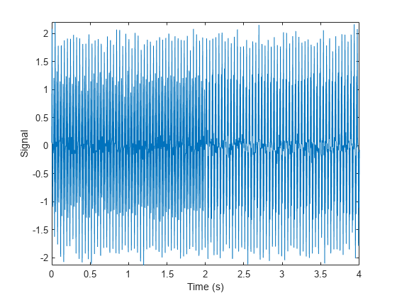
    Load and visualize a nonstationary continuous signal composed of sinusoidal waves with a distinct change in frequency. The signal is sampled at 250 Hz.

    fs = 250;
    load nonstatdistinct
    t = (0:length(nonstatdistinct)-1)/fs;
    plot(t,nonstatdistinct)
    xlabel('Time (s)')
    ylabel('Signal')
    axis tight

    Figure contains an axes object. The axes object with xlabel Time (s), ylabel Signal contains an object of type line.

    Use ewt to obtain a multiresolution analysis (MRA) of the signal.

    mra = ewt(nonstatdistinct);

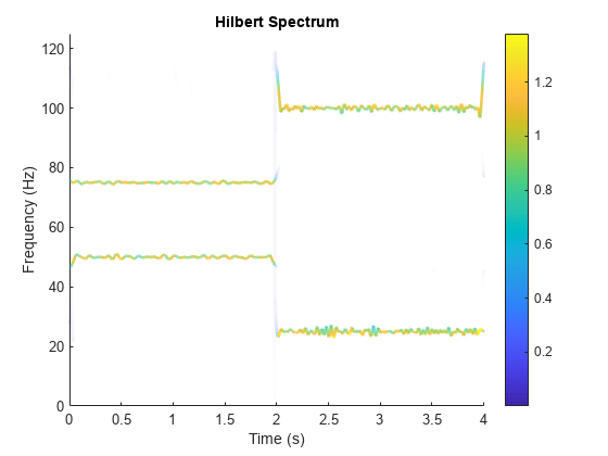
    Use the MRA components with the hht function and plot the Hilbert spectrum.

    hht(mra,fs)

    Figure contains an axes object. The axes object with title Hilbert Spectrum, xlabel Time (s), ylabel Frequency (Hz) contains 4 objects of type patch.

    The frequency versus time plot is a sparse plot with a vertical color bar indicating the instantaneous energy at each point in the MRA. The plot represents the instantaneous frequency spectrum of each component decomposed from the original mixed signal.

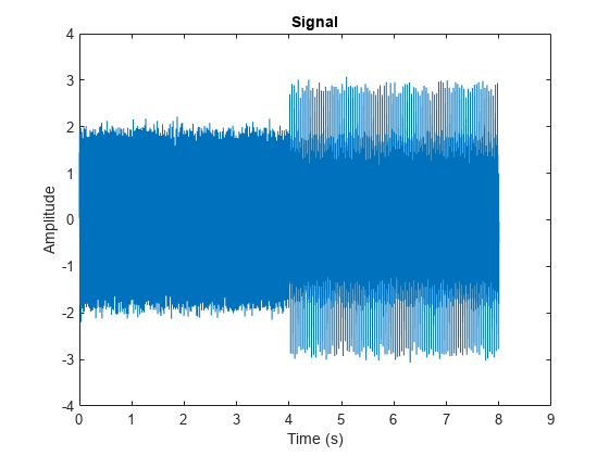
    Create a nonstationary continuous signal composed of sinusoidal waves with a distinct change in frequency. The signal is sampled at 1000 Hz.

    Fs = 1000;
    t = 0:1/Fs:4;
    x1 = sin(2*pi*50*t) + sin(2*pi*200*t);
    x2 = sin(2*pi*25*t) + sin(2*pi*100*t) + sin(2*pi*250*t);
    x = [x1 x2] + 0.1*randn(1,length(t)*2);
    t1 = (0:length(x)-1)/Fs;
    plot(t1,x)
    xlabel('Time (s)')
    ylabel('Amplitude')
    title('Signal')

    Figure contains an axes object. The axes object with title Signal, xlabel Time (s), ylabel Amplitude contains an object of type line.

    Use ewt and obtain the MRA of the signal. Display the normalized peak frequencies identified in the signal, and the approximate frequency passbands of the filter bank. Because the frequencies are in cycles per sample, normalize by the sampling frequency. Note that the peak frequencies correspond to the frequencies of the sinusoidal waves.

    [mra,~,wfb,info] = ewt(x);
    Fs*info.PeakFrequencies
    ans = 5×1
    
      249.9375
      200.0750
      100.1000
       50.1125
       25.1187
    
    
    Fs*info.FilterBank.Passbands 
    ans = 5×2
    
      223.6941  500.0000
      141.5896  223.6941
       70.8573  141.5896
       35.4911   70.8573
             0   35.4911


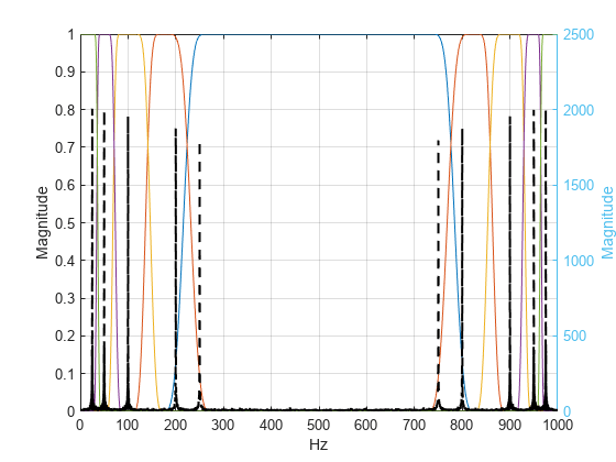
    Plot the magnitude spectrum of the signal, and the filter bank. The locations of the peaks determine the filter passbands.

    f = 0:Fs/length(x):Fs-1/length(x);
    plot(f,wfb)
    ylabel('Magnitude')
    grid on
    yyaxis right
    plot(f,abs(fft(x)),'k--','linewidth',1.5)
    ylabel('Magnitude')
    xlabel('Hz')

    Figure contains an axes object. The axes object with xlabel Hz, ylabel Magnitude contains 6 objects of type line.

    Because the empirical wavelets form a Parseval tight frame, the analysis filter bank is equal to the synthesis filter bank. Therefore, squaring the magnitudes at each frequency summed over the filters equals 1. If the sum was not equal to 1, perfect reconstruction would not be possible.

    Load an ECG signal. The signal is sampled at 180 Hz.

    load wecg

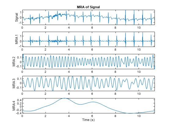
    Use ewt to obtain a multiresolution analysis (MRA) of the signal, and the corresponding analysis coefficients. Use the four largest peaks to determine the filter passbands.

    mp = 4;
    [mra,cfs] = ewt(wecg,'MaxNumPeaks',mp);

    Plot the signal and the MRA components.

    fs = 180;
    subplot(mp+1,1,1)
    t = (0:length(wecg)-1)/fs;
    plot(t,wecg)
    title('MRA of Signal')
    ylabel('Signal')
    axis tight
    for k=1:mp
        subplot(mp+1,1,k+1)
        plot(t,mra(:,k))
        ylabel(['MRA ',num2str(k)])
        axis tight
    end
    xlabel('Time (s)')

    Figure contains 5 axes objects. Axes object 1 with title MRA of Signal, ylabel Signal contains an object of type line. Axes object 2 with ylabel MRA 1 contains an object of type line. Axes object 3 with ylabel MRA 2 contains an object of type line. Axes object 4 with ylabel MRA 3 contains an object of type line. Axes object 5 with xlabel Time (s), ylabel MRA 4 contains an object of type line.

    Verify that summing the MRA components results in perfect reconstruction of the signal.

    max(abs(wecg-sum(mra,2)))
    ans = 
    8.8818e-16
    

    Verify energy preservation of the EWT analysis coefficients.

    cfsenergy = sum(sum(abs(cfs).^2));
    [cfsenergy norm(wecg,2)^2]
    ans = 1×2
    
      298.2759  298.2759


    Input Arguments

    collapse all

    Input data, specified as a real- or complex-valued vector or as a single-variable timetable containing a single column vector. x must have at least two samples.

    Data Types: single | double
    Complex Number Support: Yes

    Name-Value Arguments

    Specify optional pairs of arguments as Name1=Value1,...,NameN=ValueN, where Name is the argument name and Value is the corresponding value. Name-value arguments must appear after other arguments, but the order of the pairs does not matter.

    Before R2021a, use commas to separate each name and value, and enclose Name in quotes.

    Example: ewt(x,'MaxNumPeaks',5,'SegmentMethod','localmin') obtains the MRA of x using the five largest peaks and the first local minimum between adjacent peaks.

    Threshold percentage of maximum peak used to determine which peaks to retain in the multitaper power spectrum of x, specified as a real number in the interval (0, 100). Local maxima in the multitaper power spectral estimate of x are normalized to lie in the range [0,1] with the maximum peak equal to 1. All peaks with values strictly greater than PeakThresholdPercent of the maximum peak are retained.

    Data Types: single | double

    Segmentation method used to determine the EWT filter passbands, specified as:

    • 'geomean' — Geometric mean of adjacent peaks

    • 'localmin' — First local minimum between adjacent peaks

    If no local minimum is identified between adjacent peaks, the function uses the geometric mean.

    Maximum number of peaks used to determine the EWT filter passbands. If ewt finds fewer peaks than the number specified in MaxNumPeaks, it uses the maximum number of peaks available. If it does not find any peaks, ewt uses a level-one discrete wavelet transform (DWT) filter bank.

    You cannot specify both MaxNumPeaks and PeakThresholdPercent.

    Data Types: single | double

    Frequency resolution bandwidth of the multitaper power spectral estimate, specified as a real number less than or equal to 0.25.

    The value of FrequencyResolution determines how many sine tapers are used in the multitaper power spectrum estimate. The bandwidth of a sine multitaper power spectral estimate is (K+1)/(N+1), where K is the number of tapers and N is the length of the signal. The minimum value of FrequencyResolution is 2.5/N, where N is the maximum of the signal length and 64.

    Data Types: single | double

    Logarithm of spectrum logical used to determine the peak frequencies. If LogSpectrum is set to true, the log of the multitaper power spectrum is used. Consider setting LogSpectrum to true if using the PeakThresholdPercent segmentation method and there is a dominant peak frequency that is significantly larger in magnitude than other peaks.

    Output Arguments

    collapse all

    Multiresolution analysis (MRA), returned as a matrix or timetable.

    • When x is a vector, mra is a matrix where each column stores an extracted MRA component.

      • For real-valued x, the MRA components are ordered by decreasing center frequencies. The final column in mra corresponds to the lowpass scaling filter.

      • For complex-valued x, the MRA components start near −½ cycles per sample and decrease in center frequency until the lowpass scaling coefficients are obtained. The frequency then increases toward +½ cycles per sample.

    • When x is a timetable, mra is a timetable with multiple single variables where each variable stores an MRA component.

    See the info structure array for a description of the frequency bounds for empirical wavelet and scaling filters.

    If x has less than 64 samples, ewt works on a zero-padded version of x of length 64. The MRA components are truncated to the original length.

    EWT analysis coefficients, returned as a matrix. If the input data is real-valued, then cfs is a real-valued matrix. Otherwise, cfs is a complex-valued matrix. Each column of cfs stores the EWT analysis coefficients for the corresponding MRA component. The frequency bands of the analysis coefficients are identical to the ordering of the MRA components. If x has less than 64 samples, cfs contains the analysis coefficients obtained from the zero-padded version of x.

    Data Types: single | double

    Empirical wavelet filter bank, returned as a matrix. The center frequencies of the filters in wfb match the order in mra and cfs. Because the empirical wavelets form a Parseval tight frame, the analysis filter bank is equal to the synthesis filter bank. Therefore, summing the MRA components results in perfect reconstruction of the signal.

    Data Types: single | double

    Filter bank information, returned as a structure with the following fields:

    • PeakFrequencies — The peak normalized frequencies in cycles/sample identified in x as a column vector. For real-valued x, the frequencies are positive in the interval (0, ½) in decreasing order. For complex-valued x, the frequencies are ordered from (−½, ½). If PeakFrequencies is empty, ewt did not find any peaks and a default one-level discrete wavelet transform (DWT) subdivision is used.

    • FilterBank — A table with two variables: MRAComponent and Passbands. MRAComponent is the column index of the MRA component in mra. Passbands is a L-by-2 matrix where L is the number of MRA components. Each row of Passbands is the approximate frequency passband in cycles/sample for the corresponding EWT filter and MRA component.

    Data Types: single | double
    Complex Number Support: Yes

    References

    [1] Gilles, Jérôme. “Empirical Wavelet Transform.” IEEE Transactions on Signal Processing 61, no. 16 (August 2013): 3999–4010. https://doi.org/10.1109/TSP.2013.2265222.

    [2] Gilles, Jérôme, Giang Tran, and Stanley Osher. “2D Empirical Transforms. Wavelets, Ridgelets, and Curvelets Revisited.” SIAM Journal on Imaging Sciences 7, no. 1 (January 2014): 157–86. https://doi.org/10.1137/130923774.

    [3] Gilles, Jérôme, and Kathryn Heal. “A Parameterless Scale-Space Approach to Find Meaningful Modes in Histograms — Application to Image and Spectrum Segmentation.” International Journal of Wavelets, Multiresolution and Information Processing 12, no. 06 (November 2014): 1450044. https://doi.org/10.1142/S0219691314500441.

    Extended Capabilities

    Version History

    Introduced in R2020b