Timing Estimator
R2026bCorrelate input signal with a known reference signal and return signal timing
Since R2026b
Timing Estimator block
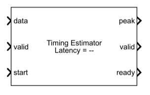
To add a block to a model, double-click the canvas and start typing the block name. Then, select the block from the list.
Libraries:
Wireless HDL Toolbox /
Synchronization
Description
The Timing Estimator block correlates your input signal with a known reference signal, detects the peak match timing, and returns the peak timing and optional signal information. The block detects peaks by computing a metric and threshold from the input signal, comparing them, and then searching a window of samples once the metric crosses the threshold. To compute the metric, the block correlates the input signal with the reference signal and computes the magnitude squared of the correlation output. To compute the threshold, the block scales the signal energy of the input from the same samples as the correlation. The block optionally returns the metric, threshold, and correlator output.
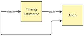
Use a timing estimator to align your input signal with a known preamble for decoding.
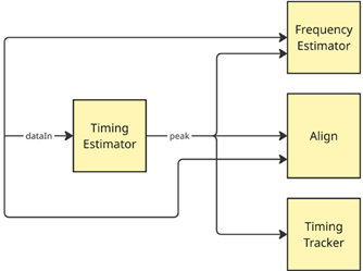
OFDM systems also use the correlator signal information from the Timing Estimator to estimate and then correct frequency offset, and the peak timing to track timing over multiple frames.
Examples
This example shows how to use the Timing Estimator block to estimate the timing offset of a known reference signal in a waveform.
The example estimates timing peaks, reports the timing offset in number of samples, and aligns the streaming waveform with the peaks for further processing. The example has a MATLAB™ reference and a Simulink™ model. The MATLAB reference explores the design space and provides test vectors. The Simulink model simulates the fixed-point and latency behavior and generates HDL code.
Generate Test Waveform
Generate a waveform containing a reference signal to use for testing timing estimation.
Generate a length-127 Zadoff-Chu sequence.
Convert to the time-domain with a 256-point IFFT.
Extend the waveform with zeros.
rng('default');

sampleRate = 100e6;

% Zadoff-Chu
fftLength = 256;
zadoffChuLength = 127;
syncSeq = zadoffChuSeq(25,zadoffChuLength);

% Convert to time-domain
freqPreambleSymbols = zeros(fftLength,1);
gridOffset = floor((fftLength-zadoffChuLength)/2);
freqPreambleSymbols((1:length(syncSeq)).'+gridOffset) = syncSeq;
preambleSymbols = ifft(fftshift(freqPreambleSymbols));

% Extend waveform with zeros
rxWaveform = [preambleSymbols; zeros(1000,1)];
Add channel impairments to the waveform.
Add a timing offset with an integer and fractional component.
Add white Gaussian noise.
Normalize the waveform to use the full range of the input fixed-point type.
% Timing offset
channelTOffset = 142.6;

channelFracOffset = channelTOffset-floor(channelTOffset);
chanDelayFIR = designFracDelayFIR(FractionalDelay=channelFracOffset,Bandwidth=2/3);
fracDelay = grpdelay(chanDelayFIR);
channelIntOffset = floor(channelTOffset) - floor(fracDelay(1));

rxWaveform = [zeros(channelIntOffset,1); rxWaveform];
rxWaveform = filter(chanDelayFIR,1,rxWaveform);

% AWGN
SNRdB = 5;
SNR  = 10.^(SNRdB/10);
sigPower = 1/(fftLength*fftLength/zadoffChuLength);
rxWaveform = awgn(rxWaveform,SNR,sigPower,"linear");

% Normalize rxWaveform
rxWaveform = 0.875 * rxWaveform ./ max(abs(rxWaveform));
Define Block and MATLAB reference constants
Define constants required to perform the timing offset estimation. These values are used in the MATLAB reference code and to set block properties in the Simulink model.
Timing Estimator
refSignal: Set Reference signal to match the expected preamble symbols. The reference signal is normalized to preserve power across the correlator.oversampleFactor: Set Minimum number of cycles between valid input samples to 1 because the input data is continuously valid.thresholdBackoff_dB: Set Backoff (dB) to provide a trade-off between sensitivity and false detections.thresholdFloor: Set Floor to avoid false detections when the signal power is very low. Designed for a noise floor at ±2^-12, corresponding to a 12-bit ADC.peakWindowLength: Set Window length to perform a small search for spread peaks when multiple samples cross the threshold.
Stream Aligner
tEstLatencyCycles: Calculate the latency of the Timing Estimator in clock cycles to compute the stop time for Simulink.tEstLatencySamples: Calculate the latency of the Timing Estimator in samples to computealignBufferSize.alignOffset: Set the offset to align timing estimator peaks with the start of the reference signal after alignment.alignBufferSize: Set the size of the buffer in theStream Alignerfrom the sample latency of the Timing Estimator and the alignment offset.
% Timing Estimator
refSignal = preambleSymbols.'/sqrt(preambleSymbols'*preambleSymbols);
oversampleFactor = 1;

thresholdBackoff_dB = 3;
thresholdFloor = length(refSignal) * (2^-12).^2;

peakWindowLength = 3;

% Stream Aligner
[tEstLatencyCycles,tEstLatencySamples] = timingEstimatorLatency(~isreal(rxWaveform),refSignal,oversampleFactor,peakWindowLength);

alignOffset = length(refSignal)-1;
alignBufferSize =  2^nextpow2(tEstLatencySamples+alignOffset);
Run MATLAB Reference
Run the MATLAB reference code to verify the algorithm and provide test vectors for Simulink.
% Correlation metric
corrWeights = fliplr(conj(refSignal));

metricML = abs(filter(corrWeights,1,rxWaveform)).^2;

% Threshold
thresholdPrescale = sqrt(10^(-thresholdBackoff_dB/10) * sum(abs(corrWeights).^2));
rxWaveformPrescale = rxWaveform*thresholdPrescale;

refSignalLength = length(refSignal);
thresholdFilt = ones(refSignalLength,1);
thresholdML = filter(thresholdFilt,1,abs(rxWaveformPrescale).^2);
thresholdML(thresholdML<thresholdFloor) = thresholdFloor;

% Determine where the threshold is exceeded
exceedsML   = metricML > thresholdML;
survivors = metricML .* exceedsML;
exceedingIndices = find(exceedsML);

% Keep track of where the search is resumed after each trigger.
resumeIndex = 1;

% Store information about detected peaks.
peakInfoML = [];

% For each point at which the correlation level exceeds the threshold
for n=1:size(exceedingIndices,1)
    triggerIndex = exceedingIndices(n);

    % Only trigger the detector if the resume index has been reached.
    if triggerIndex >= resumeIndex
        if triggerIndex+peakWindowLength-1 > size(survivors,1)
            warning("Peak detector window overruns the end of the waveform. Run with more data to detect the peak.")
            break;
        end

        % Perform a local search for the peak across peakWindowLength samples starting from the trigger point.
        [~,peakSubIndex] = max(survivors(triggerIndex:triggerIndex+peakWindowLength-1));
        peakIndex        = triggerIndex + peakSubIndex - 1;

        peak.Metric = metricML(peakIndex);
        peak.Threshold = thresholdML(peakIndex);
        peak.tOffset = peakIndex-1;
        peakInfoML = [peakInfoML; peak]; %#ok<AGROW>

        % Move the resume index to prevent further triggering until the search window has been passed.
        resumeIndex = triggerIndex + peakWindowLength;
    end
end

% Adjust peak tOffsets by the alignOffset so tOffset is relative to the aligned data
for ii = 1:numel(peakInfoML)
    peakInfoML(ii).tOffset = peakInfoML(ii).tOffset-alignOffset;
end
Run Simulink Model
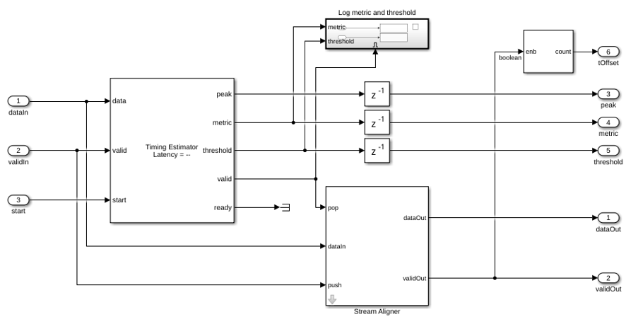
The model implements the timing offset estimation algorithm by using the Timing Estimator block, and aligns the input waveform to the latency of the Timing Estimator with the Stream Aligner subsystem. The Stream Aligner subsystem also offsets the data stream by the length of the reference signal minus one. This re-aligns the timing estimator peaks from the end of the reference signal in the received waveform to the start. A 64-bit counter counts the valid samples after alignment, to report the timing offset as an absolute number of samples into the aligned waveform.
The image shows the Estimate Timing Offset subsystem.
model = "estimateTimingOffset";
load_system(model);
set_param(model+"/Estimate Timing Offset",Open='on');
Simulate the Simulink model using the same input signals as MATLAB and read results back for comparison.
stopTime = (length(rxWaveform)+tEstLatencyCycles-1)./sampleRate;
outSL = sim(model);

metricSL = double(outSL.metric);
thresholdSL = double(outSL.threshold);

peakInfoMetricSL = num2cell(double(outSL.peakMetric));
peakInfoThresholdSL = num2cell(double(outSL.peakThreshold));
peakInfotOffsetSL = num2cell(double(outSL.peaktOffset));
peakInfoSL = struct('Metric',peakInfoMetricSL,'Threshold',peakInfoThresholdSL,'tOffset',peakInfotOffsetSL).';
Display Results
Analyze the outputs to verify the algorithm behavior. Compare MATLAB and Simulink results to confirm the equivalence and see the fixed-point quantization error.
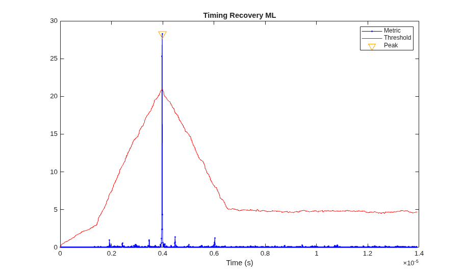
To see the location of peaks in the waveform, plot timing recovery metric and threshold in MATLAB.
Display the peaks detected in MATLAB and Simulink, and the expected timing offset from the channel configuration. The detected peak timing offsets can vary by ±1 relative to the expected value due to the fractional offset.
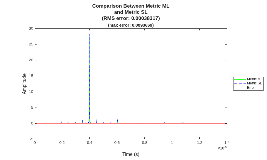
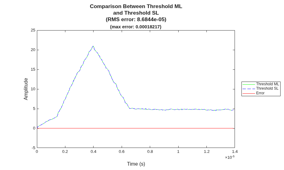
Plot comparisons between the metric and threshold signals between MATLAB and Simulink.
figure(1); clf
n = 0:length(metricML)-1;
x = n.'/sampleRate;
plot(x,metricML,'.-b'); hold on;
plot(x,thresholdML,'r');
plot(x([peakInfoML.tOffset]+alignOffset+1),[peakInfoML.Metric],"v",'MarkerSize',10,'MarkerEdgeColor','#FFA500');
hold off;
xlabel("Time (s)");
title("Timing Recovery ML");
legend("Metric","Threshold","Peak");

disp("Expected tOffset from channel: " + num2str(channelTOffset + length(corrWeights) - 1 - alignOffset) + newline);

disp("Detected peaks ML:" + newline)
disp(struct2table(peakInfoML))

disp("Detected peaks SL:" + newline)
disp(struct2table(peakInfoSL))

figure(2); clf;
plotSignalComparison(metricML,metricSL,"Metric ML","Metric SL",sampleRate);

figure(3); clf;
plotSignalComparison(thresholdML,thresholdSL,"Threshold ML","Threshold SL",sampleRate);
Expected tOffset from channel: 142.6

Detected peaks ML:

    Metric    Threshold    tOffset
    ______    _________    _______

    28.258     20.964        143

Detected peaks SL:

    Metric    Threshold    tOffset
    ______    _________    _______

    28.254     20.964        143
Extended Examples
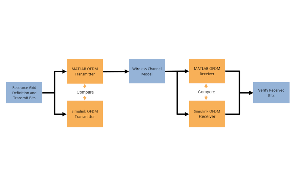
Introduction to Custom OFDM
The design and verification of a transmitter and receiver for a custom OFDM communication system that is suitable for HDL code generation.
QPSK Transmitter and Receiver
Design and verify a QPSK transmitter and receiver for hardware.
Ports
Input
Output
Parameters
Algorithms
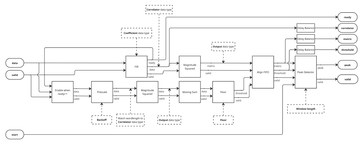
This diagram shows the internal architecture of the Timing Estimator block. The
data and valid inputs feed an FIR filter. The
filter is a Discrete FIR Filter block that implements the
correlation of the input with your Reference signal,
flip(conj(refSignal)). The filter is configured with Filter
structure set to Partly serial systolic, your setting
for Minimum number of cycles between valid input samples, and your
setting for the Coefficient data type. The output of the filter is
quantized to the Correlator data type.
The design calculates the metric output by squaring the magnitude of the filter output. This value is quantized to the Output data type.
The prescale step implements
sqrt(10^(-Backoff/10)*sum(abs(refSignal).^2)), using the value you
specify in the Backoff parameter. The design quantizes the output of the
prescale to the same word length as the Correlator data type, then
squares the magnitude and quantizes to the Output data type. A moving sum
over length(refSignal) calculates the threshold energy for input to the
peak detector, and the floor calculation sets the lowest power level to the
Floor parameter value.
The peak detector compares the scaled input signal energy, threshold,
with the correlation power, metric. Once the threshold is met, the peak
detector searches a window of samples for the highest power and returns
peak set to true on that cycle.
Extended Capabilities
Version History
Introduced in R2026b

