Spectrum Visualization on NI USRP Radio

Since R2024b

Deploy and verify a real-time, wideband spectrum visualization algorithm on the FPGA of an NI™ USRP™ radio. The algorithm synchronizes data streams from two antennas to produce a spectrogram with twice the bandwidth that a single antenna can achieve.

Workflow

In this example, you follow a step-by-step guide to generate a custom FPGA image from a Simulink^® model and deploy it on an NI USRP radio by using a generated MATLAB^® host interface script.

For more information about how to prototype and deploy software-defined radio (SDR) algorithms on the FPGA of an NI USRP radio, see Target NI USRP Radios Workflow.

Design Overview

The example uses a design that does the following:

Synchronizes two input data streams captured over the air on two independent antennas.
Performs a fast Fourier transform (FFT) on each input data stream.
Calculates the spectrum density of each input data stream.
Packages the processed data to send to the host.

Requirements

To target NI USRP radio devices with Wireless Testbench™, you must install and configure third-party tools and additional support packages.

For details about which NI USRP radios you can target, see Supported Radio Devices.

Note

Generating a bitstream with this workflow is supported only on a Linux^® operating system (OS). For details about host system requirements, see System Requirements.

For details about how to install and configure additional support packages and third-party tools, see Installation for Targeting NI USRP Radios.

Note

If you use this example with a USRP E320 radio, hardware limitations require you to take additional steps:
- Only one center frequency can be configured across both receive antennas. The output data contains two sets of data captured at the same center frequency. When you use the live script to plot the data, disregard the left side of the plot.
- This example uses one transmit antenna and two receive antennas. This configuration is not supported on a USRP E320 radio. Before you run the VerifySpectrumVisualizationAlgorithmUsingMATLABExample.m script, you must adjust the TransmitAntennas property on the usrp System object™ to select both transmit antennas. If you want to transmit a waveform, you must also modify the transmitSignal variable to send zero data on the second channel.
If you use this example with a USRP X310 radio with TwinRX daughterboards, you cannot use your radio to transmit a test tone. To verify the design running on your radio by using a transmitted tone, use an external transmitter.

Set Up Environment and Radio

Set up a working directory for running the example by using the openExample function in MATLAB. This function downloads the example files into a subfolder of the Examples folder in the currently running release and then opens the example. If a copy of the example exists, openExample opens the existing version of the example.

openExample('wt/SpectrumVisualizationOnNIUSRPRadioExample')

The working directory contains all the files you need to use this example, including helper functions and files. The files you interact with are:

wtSpectrumVisualizationSL.slx — The Simulink hardware generation model. This model includes the design under test (DUT) subsystem, which implements a spectrum visualization algorithm, and additional subsystems than enable you to simulate the DUT behavior.
SpectrumVisualizationOnNIUSRPRadioExample.m — The MATLAB script that you can use to simulate the behavior of the Simulink model before you generate HDL code.
VerifySpectrumVisualizationAlgorithmUsingMATLABExample.m — The live script that you use in MATLAB to verify the algorithm running on your radio.

To program the FPGA on your radio with the bitstream that you generate in this example, and to verify the algorithm running on your radio, use the Radio Setup wizard to connect and set up your radio.

Simulink Hardware Generation Model

This example uses:

Open Script

The Simulink model in this example is a hardware generation model of an SDR algorithm. Using the HDL Code tab in the Simulink Toolstrip or the HDL Workflow Advisor, you can generate a custom HDL IP core from the model, then generate a bitstream and load it onto the FPGA on your radio. You can then generate a host interface script that provides the MATLAB code you need to interact with the hardware.

Open Model

Open the Simulink model.

modelname = 'wtSpectrumVisualizationSL';
open_system(modelname);

The top level model, wtSpectrumVisualizationSL, includes three subsystems:

The SpectrogramBlock subsystem implements the spectrum visualization algorithm. This subsystem is the device under test (DUT).
The RadioRFSource subsystem simulates the radio front end to provide a test input to the DUT.
The MatlabHostInterface subsystem simulates the connections between the host and the DUT, including register and streaming interfaces.

Open the SpectrogramBlock subsystem.

open_system([modelname '/SpectrogramBlock']);

The data streaming inputs from the radio to the DUT are int16 complex numbers that have been quantized by an analog-to-digital converter in the radio front end. The FFTs block does the following to calculate the power spectral density of the input streams:

Computes a 1024-point FFT for both input data streams.
Calculates the square of the FFT to give the power spectral density of the RF signal received by each antenna. The unit of power is arbitrary and is not normalized to the frequency resolution.
Converts the resulting power to floating point to enable it to be efficiently converted to a dB value relative to an arbitrary power value of 1.
Quantizes the result to 8 bits, which is 128 bins.

The FFTs block has several write register ports that control the quantization. The Level0 and Level1 inputs control the power level of the spectrum output of each stream. The Amp0 and Amp1 inputs control the spectrum power resolution of each stream. The FrameNum input controls how many frames to receive in each read from the host.

The DensityCalculationController block accumulates the power calculated in the FFTs block to produce a histogram. The total number of bins is the length of the FFT multiplied by the number of quantized bins, which is 1024 * 128. In each iteration of the accumulation, 1 is added to each bin that corresponds to the power level measured at that FFT point. There are 16 iterations for each frame of data, so the range of output values for each bin is between 0 and 16. When the host plots this data as a histogram, each value corresponds to a color ranging from cool to warm. The accumulated data for each data stream is stored in a RAM block, RAM0 and RAM1.

Finally, the DataPackager block packages the concatenated spectrum density data frames. The raw streams of output data are formatted into packets that conform to the simplified AXI-stream protocol. The output packet length is 256 samples, which is the recommended value. For more information, see Simplified AXI-Stream Protocol. The timestamp from the hardware is latched every time the DataPackager sends data to the host.

To ensure synchronization between the two streams of RF data, the sync_streamers block performs an AND operation on the two valid_in signals from the input stream port. The result of this operation is sent back to both ready_out ports, which guarantees that the two data streams are synchronized. In addition, a ready_override input is added to override the ready signal of the DUT. The ready_override signal is asserted during the transition period when data streaming is started or stopped. This prevents an interlock between the two data streamers, which ensures that the internal buffers do not overflow.

The timestamp can be read from TSOut0H and TSOut0H as the lower and higher 32-bit integer of the 64-bit timestamp. Since the two input streams are synchronized, their timestamps are the same. For this reason, only TS0 and HasTime0 are used by the TSLatch block to produce the DUT timestamp output. The HasTime0 input port indicates that there is a timestamp.

Simulate Design

To simulate the model, a band-limited noise signal is generated using a random number generator and a low-pass filter. This signal is the input signal to both stream ports simultaneously. You can visualize the output by using the hPlotSimulationResult helper function. Four frames of data are plotted for visual verification of each port.

Verify the design by simulating the model.

sl_out = sim(modelname);

Use the hPlotSimulationResult helper function to plot the output data.

hPlotSimulationResult(sl_out);

The output shows four spectrums of low-pass filtered noise from stream port 0 and stream port 1. The results from each stream are identical and match the stimulus data. In the hardware implementation, each antenna receives distinct signals in adjacent frequency bandwidths that are received by the two stream ports. This setup doubles the bandwidth for spectrum visualization.

Configure IP Core

When you are satisfied with the simulated behavior of the model, you can proceed to integrate your design into a custom IP core by generating HDL code and mapping the model inputs and outputs to the hardware interfaces.

First, use the hdlsetuptoolpath (HDL Coder) function to set up the tool chain. Specify the path to your Vivado^® bin directory. For more information, see Set Up Third-Party Tools.

hdlsetuptoolpath('ToolName','Xilinx Vivado', ...
    'ToolPath','/opt/Xilinx/Vivado/2021.1/bin');

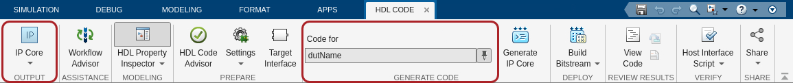
From the Apps tab in the Simulink Toolstrip, select HDL Coder. Then open the HDL Code tab.

Configure Output Options

In the HDL Code tab, configure the output options:

Ensure the SpectrogramBlock subsystem is pinned in the Code for option. To pin this selection, select the SpectrogramBlock subsystem in the Simulink model and click the pin icon.
Select IP Core as the Output > IP Core option.

HDL Code tab in the Simulink Toolstrip

Configure HDL Code Generation Settings

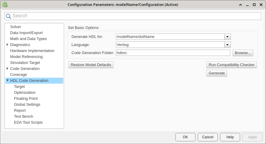
Open the Configuration Parameters dialog box by clicking Settings in the HDL Code tab.

In the HDL Code Generation pane, ensure that Language is set to Verilog. By default, HDL Coder generates the Verilog^® files in the hdlsrc folder. You can select an alternative location. If you make any changes, click Apply.

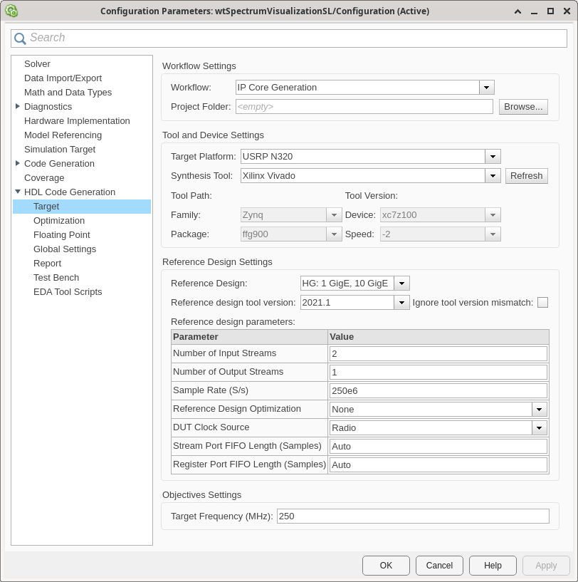
HDL Code Generation panel in the Configuration Parameters window

In the Target pane, configure these settings:

Under Workflow Settings, select the IP Core Generation workflow. To set Project Folder, click Browse and select a target location for saving the generated project files. If you do not specify a project folder, the software saves the generated project files in the working directory.
Under Tool and Device Settings, select your radio from the Target Platform list. This example uses a USRP N320 radio. If you are using a different radio, adjust the reference design parameters accordingly.
Under Reference Design Settings, set Reference Design to the desired reference FPGA image for your design, based on how you set up your hardware. For a USRP N320 radio, you have one option: HG: 1GigE, 10GigE.
Set the reference design parameters to these values:
- Number of Input Streams — Set to 2 because the DUT is connected to two parallel data input streams.
- Number of Output Streams — Set to 1 because the DUT is connected to one data output stream.
- Sample Rate (S/s) — Set to the maximum supported master clock rate for the target device. This value is set by default. For an N320 radio, this value is 250e6. To determine which sample rates are available for your radio, see Determine Radio Device Capabilities.
- Reference Design Optimization — Set to None. This example uses a simple design that does not require optimizations to meet timing constraints.
- DUT Clock Source — Set to Radio. When you select this setting, the DUT is clocked at the MCR used by the radio to achieve the specified sample rate. Alternatively, you can set this setting to Custom to set the DUT clock frequency to a user-defined value in the Target Frequency parameter under Objectives Settings.
- Stream Port FIFO Length (Samples) — Set to Auto. This setting automatically calculates the buffer length for each DUT input and output data streaming port.
- Register Port FIFO Length (Samples) — Set to Auto. This setting automatically calculates the buffer length for each DUT register port.
Under Objectives Settings, since the DUT Clock Source is set to Radio, the Target Frequency is fixed at the highest supported MCR of the radio.

HDL Code Generation > Target panel in the Configuration Parameters window

To apply these settings and close the Configuration Parameters window, click OK.

For more information, see Configure HDL Code Generation Settings.

Map Target Interfaces

In the HDL Code tab, click Target Interface to open the Interface Mapping table in the IP Core editor. To populate the table with your user logic, click the Reload IP core settings button: .

IP Core Interface Mapping table

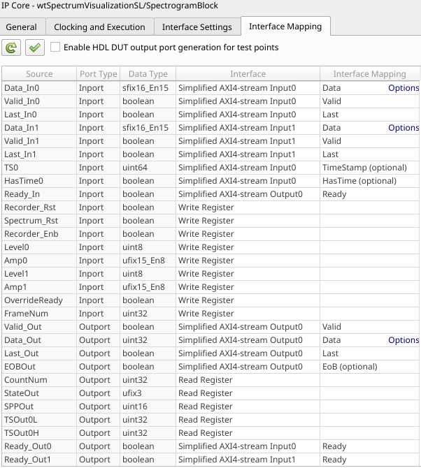
The Source, Port Type, and Data Type columns are populated based on the Simulink model. The Interface column automatically populates based on the port names in your model:

The input register ports map to Write Register interfaces.
The output register ports map to Read Register interfaces.
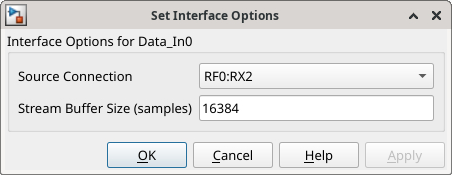
The Data_In0, Valid_In0, Last_In0, HasTime0, TS0, and Ready_Out0 ports map to a Simplified AXI4-stream Input0 interface.
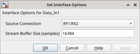
The Data_In1, Valid_In1, Last_In1, and Ready_Out1 ports map to a Simplified AXI4-stream Input1 interface.
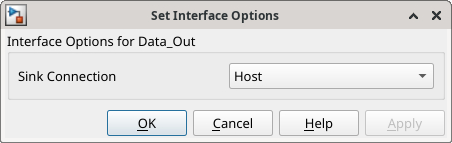
The Data_Out, Valid_Out, Last_Out, EOBOut, and Ready_In ports map to a Simplified AXI4-stream Output0 interface.

The Interface Mapping column is populated automatically based on the port names in the model.

To set the interface options for the streaming interfaces, open the Set Interface Options window by clicking Options in the far right of the table.

Set the stream buffer size to 32768, which is the default setting. The buffer size must be a power of two to ensure optimal use of the FPGA RAM resources. The buffer size is specified in terms of the number of samples, with each sample having a size of 8 bytes.

For the Data_In0 and Data_In1 options, select a receive antenna as the source connection. The DUT receives input samples from these antenna on the radio. Select antennas with independently tunable center frequencies.

If you are using a USRP E320 radio, the only two available antennas cannot be configured with independent center frequencies. Choose the two antennas that are available on your radio.
If you are using a USRP N310 radio, RF0:RX2 and RF1:RX2 share a center frequency, as do RF2:RX2 and RF3:RX2. Choose antennas that do not share a center frequency.

Set the stream buffer size to 16384. This value is lower than the default setting to reduce the hardware resources required and enable the design to meet timing requirements. The buffer size must be a power of two to ensure optimal use of the FPGA RAM resources. The buffer size is specified in terms of the number of samples, where each sample has 8 bytes.

Set Interface Options dialog box for Data_In0, showing source connection set to RF0:RX2 and stream buffer size set to 16384 samples

Set Interface Options dialog box for Data_In0, showing source connection set to RF1:RX2 and stream buffer size set to 16384 samples

For the Data_Out options, select the host as the sink connection. The DUT streams samples directly to MATLAB for post-processing.

Set Interface Options dialog for Data_Out, showing sink connection set to Host.

When you have populated the table, validate the interface mapping by clicking the Validate IP core settings button: .

For more information, see Map Target Interfaces.

Generate and Load Bitstream

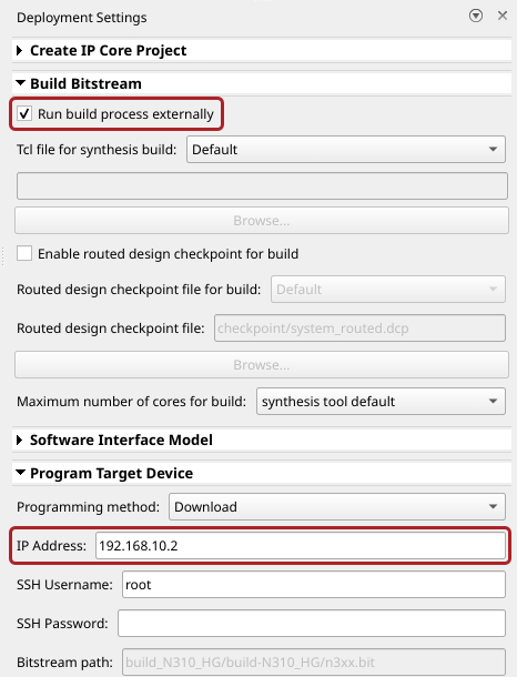
To generate a bitstream from the configured IP core, first open the deployment settings from the Build Bitstream button.

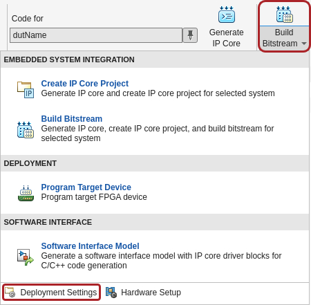
Deployment Settings button in Build Bitstream drop-down menu

Ensure that the Run build process externally option is selected. This setting is the default and it ensures that the bitstream build executes in an external shell, which allows you to continue using MATLAB while building the FPGA image.
In the Program Target Device settings, set the IP address. The default is 192.168.10.2. If your radio has a different IP address, update this field with the correct value.

Deployment Settings window

Click Build Bitstream to create a Vivado IP core project and build the bitstream. After the basic project checks complete, the Diagnostic Viewer displays a Build Bitstream Successful message along with warning messages. However, you must wait until the external shell displays a successful bitstream build before moving to the next step. Closing the external shell before this time terminates the build.

The bitstream for this project generates with the name n3xx.bit and is located in the build_N320_HG/build_N320_HG folder of the working directory after a successful bitstream build. If you are using a different radio, the name and location reflects your radio.

To load the bitstream onto the device now, click Program Target Device from the Build Bitstream button. Alternatively, you can load the bitstream later by using the programFPGA function in the generated host interface script.

For more information, see Generate Bitstream and Program FPGA.

Generate Host Interface Scripts

To generate MATLAB scripts that enable you to connect to and run your deployed design on your radio, in the HDL Code tab, click Host Interface Script. This step generates two scripts in your working directory based on the target interface mapping that you configured for your IP core.

gs_wtSpectrumVisualizationSL_interface.m — Host interface script that creates an fpga object for interfacing with your DUT running on the FPGA from MATLAB. The script contains code that connects to your hardware and programs the FPGA and code samples to get you started with running the algorithm on your radio. For more information, see Interface Script File.
gs_wtSpectrumVisualizationSL_setup.m — Setup function that configures the fpga object with the hardware interfaces and ports from your DUT algorithm. The function contains DUT port objects that have the port name, direction, data type, and interface mapping information, which it maps to the corresponding interfaces. For more information, see Setup Function File.

Edit Setup Function File

In the generated setup function file, the streaming interfaces are configured with the default frame size and timeout values, which are 1e5 samples and 1+(FrameSize/SampleRate) seconds, respectively. Before you run the host interface script, manually update these values.

Open the setup function file for editing.
```
edit gs_wtSpectrumVisualizationSL_setup.m
```
Identify the call to the addRFNoCStreamInterface function for the data output port.
Update the FrameSize value to 32798*8, which is equal to 8 packets of output data from the spectrum visualization model.
Note
If you have a 10 Gigabit Ethernet network connection, you can increase the number of packets per frame. If you increase this value, you must also update the hhPlotSpectrumScroll helper function to use the same value.

Update the Timeout value to 1.5 to increase the system robustness if your network connection has limited bandwidth.

addRFNoCStreamInterface(hFPGA, ...
   "InterfaceID", "RX_STREAM#0", ...
   "Streamer", "0/RX_STREAM#0", ...
   "Direction", "OUT", ...
   "FrameSize", 32768*8, ...
   "Timeout", 1.5);

Save the updated setup function file.

Verify Spectrum Visualization Algorithm Using MATLAB

This example uses:

Open Live Script

To verify the algorithm running on your radio, use this modified version of the host interface script to setup the device, create a UI figure, and visualize the spectrum in real time using MATLAB.

Open Live Script

You can open this live script in MATLAB from the example working directory and use it interactively. In the Files panel, navigate to your example working directory and open VerifySpectrumVisualizationAlgorithmUsingMATLABExample.m.

Select Radio

Call the radioConfigurations function. The function returns all available radio setup configurations that you saved using the Radio Setup wizard.

savedRadioConfigurations = radioConfigurations;

To update the menu with your saved radio setup configuration names, click Update. Then select the radio to use with this example.

savedRadioConfigurationNames = [string({savedRadioConfigurations.Name})];
radioConfig = savedRadioConfigurationNames(1) ;

Evaluate independent receive antennas available on your radio device. You select DUT input antenna connections from the available options later in the script.

[independentReceiveAntenna1, IndependentReceiveAntenna2] = hIndependentFrequencyCaptureAntennas(radioConfig);

Evaluate the transmit antennas available on your device. You select a transmit antenna for transmitting a tone from the available options later in the script.

transmitAntennas = hTransmitAntennas(radioConfig);

Create Radio Object

Use the radioConfigurations function with the configuration name to create a radio object.

radio = radioConfigurations(radioConfig);

Create usrp System Object

Create a usrp System object™ with the specified radio. This System object controls the radio hardware.

hDevice = usrp(radio);

Program FPGA

If you have not yet programmed your device with the bitstream, select the load bitstream option to use the programFPGA function. Update the code with your bitstream and device tree file. You can find these files in the programFPGA call in the generated host interface script, gs_wtSpectrumVisualizationSL_interface. If your radio is a USRP X310, you need only a bitstream file to program the FPGA.

loadBitstream = false;
if(loadBitstream)
programFPGA(hDevice, ...
    "build_N320_HG/build-N320_HG/n3xx.bit", ...     % replace with your .bit file
    "build_N320_HG/build/usrp_n320_fpga_HG.dts");   % replace with your .dts file
end

To configure the DUT interfaces according to the hand-off information file, use the describeFPGA function. Calling this function additionally sets the default values for the SampleRate, DUTInputAntennas, and DUTOutputAntennas properties based on the selections you made in Simulink.

% Replace with your hand-off information file
describeFPGA(hDevice,"wtSpectrumVisualizationSL_wthandoffinfo.mat");

Configure Device

Configure the usrp System object to specify the sample rate, antennas, and antenna gain values.

To obtain the maximum sample rate available for your radio, use the hMaxSampleRate helper function. Set the SampleRate property on the usrp System object to the maximum sample rate.

maxSampleRate = hMaxSampleRate(radioConfig);
hDevice.SampleRate = maxSampleRate;

To obtain the maximum instantaneous bandwidth available for your radio, use the hMaxBandwidth helper function. You use this value later to generate the UI figure.

maxBandwidth = hMaxBandwidth(radioConfig);
singleAntennaBandwidth = maxBandwidth;

Set the DUTInputAntennas property to a value that corresponds to two antennas that support different center frequencies on your radio device.

If you are using a USRP E320 radio, both channels use the same center frequency. Choose both available antennas and disregard one half of the spectrum plot.
If you are using a USRP N310 radio, RF0:RX2 and RF1:RX2 share a center frequency, as do RF2:RX2 and RF3:RX2. Choose antennas that do not share a center frequency.

hDevice.DUTInputAntennas = [independentReceiveAntenna1(1),IndependentReceiveAntenna2(1)];

Specify the gain for each antenna.

hDevice.ReceiveRadioGain = [30, 30];

Select a transmit antenna that you will use to transmit a test signal to verify the operation of the spectrum visualization block. Then, specify the transmit antenna gain. If you are using a USRP E320 radio, select two transmit antennas.

hDevice.TransmitAntennas = transmitAntennas(1); 
hDevice.TransmitRadioGain = 20;

Create and Set Up FPGA Object

To connect to the DUT on the FPGA of your radio, create an fpga object with the your usrp System object device.

hFPGA = fpga(hDevice);

Set up the fpga object using the generated setup function gs_wtSpectrumVisualizationSL_setup. If you have not updated this file to set the frame size to 32798*8, return to Edit Setup Function File.

gs_wtSpectrumVisualizationSL_setup(hFPGA);

Set Up Device Object

To establish a connection with the radio hardware, call the setup function on the usrp System object. This action connects to the radio, applies the radio front end properties, and validates that the bitstream file matches the hand-off information file.

setup(hDevice);

Configure DUT

Use the writePort function to set the number of frames that the DUT outputs to 8. This value must correspond to the values used in the setup function, gs_wtSpectrumVisualizationSL_setup.m, and the hPlotSpectrumScroll helper function.

writePort(hFPGA,"FrameNum",8);

Reset the system.

writePort(hFPGA,"Recorder_Enb",0);
writePort(hFPGA,"Recorder_Rst",1);
writePort(hFPGA,"Spectrum_Rst",1);
writePort(hFPGA,"Spectrum_Rst",0);

Create and Interact With UI Figure

To create a UI figure to interact with the spectrum visualization in real-time, run the hCreateUIFigure.m script to create the spectrum visualization UI figure.

hCreateUIFigure

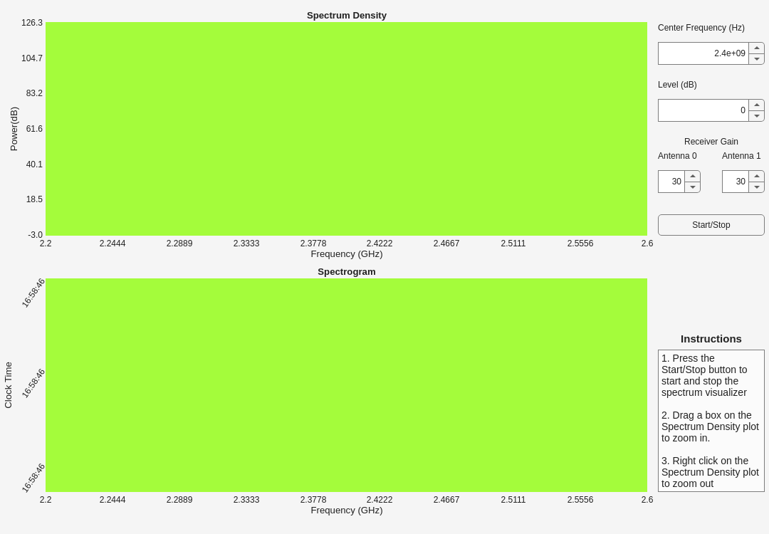
Figure Spectrogram on USRP contains 2 axes objects and other objects of type uilabel, uispinner, uibutton, uitextarea. Axes object 1 with title Spectrum Density, xlabel Frequency (GHz), ylabel Power(dB) contains an object of type image. Axes object 2 with title Spectrogram, xlabel Frequency (GHz), ylabel Clock Time contains an object of type image.

Start and Stop Spectrum Visualization

To start or stop live spectrum monitoring, click Start/Stop.

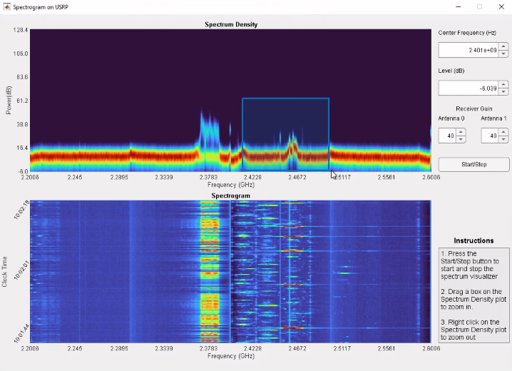
Zoom in to A Signal of Interest

To zoom in to a signal of interest, click and drag a box around the signal in the spectrum density plot. The script automatically recalculates and applies a new sample rate and scaling value to the hardware to fit the drag box. This adjustment allows for the visualization of the signal with a higher frequency and power resolution. To zoom out, right-click on the spectrum density plot. This applies the highest supported sample rate to the hardware to revert to the lowest resolution but highest bandwidth.

Horizontal spectrum density and spectrogram plots showing spectrum density versus frequency, with colored bands indicating signal strength. On the right hand side, there is a panel with controls for adjusting center frequency, level, and receiver gain are present, along with instructions for interacting with the plot. The cursor shows how to zoom in to a signal of interest.

Change Signal Level

To adjust the minimum y-axis value, use the Level setting.

Change Center Frequency

To adjust the center frequency, use the Center Frequency setting. This selects the center frequency for the plot, which is obtained on two antennas to achieve a wider bandwidth. The center frequency that must be set for each antenna is equal to the center frequency you select, plus or minus half the bandwidth of a single antenna. When you update the center frequency, the script will automatically calculate and apply the corresponding center frequencies to each antenna.

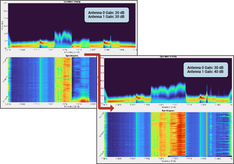
Tune Antenna Receive Gain

In some scenarios, a mismatch in the signal reception between the two receive antennas may cause a discontinuity in the plot. For example, the figure shows a plot where the amplitude of signal the lower half of the frequency axis is much larger than the amplitude of the signal in the upper half of the frequency axis. This can be caused by physical differences between the connected antennas.

To compensate for this difference, tune the Receiver Gain of the two antennas until the signal amplitude appears uniform across the frequency axis.

Side-by-side spectrum visualization plots that show how to tune the antenna gains to equalise the signal magnitude across both antennas.

Transmit Tone

To verify that the spectrum visualization algorithm on the FPGA of your radio is working as expected, first transmit a tone. Generate a tone signal at 1/4 of the current sample rate and transmit the tone over the air using the transmit function.

If you are using a USRP E320 radio, transmit zeros on the second transmit antenna. If you are using a USRP X310 radio with TwinRX daughterboards, use an external transmitter.

transmitSignal = exp(1i*2*pi/4 * (1:10000));
transmitSignal = int16(32767*transmitSignal).';

% For E320 transmission on two channels
if strcmp(radio.Hardware,"USRP E320")
    transmitSignal = [transmitSignal zeros(length(transmitSignal),1)];
end

hDevice.TransmitCenterFrequency = 2400000000;
transmit(hDevice,transmitSignal,"continuous");

Use the UI figure to view the spectrum data and verify that the deployed design is working as expected.

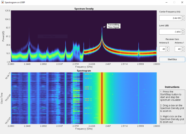
Spectrum visualization plot showing a transmitted tone at around 2.4 GHz.

After transmitting the signal, you will see a tone at 1/4 of the sample rate, near the transmit center frequency. Note that if you zoom in the transmission will stop until you transmit again.

Close the UI Figure

Close the UI figure. This automatically releases the hardware.