What Is Model Reference Adaptive Control? | Data-Driven Control
From the series: Data-Driven Control
Brian Douglas
Use an adaptive control method called model reference adaptive control (MRAC). This controller can adapt in real time to variations and uncertainty in the system that is being controlled.
See how model reference adaptive control cancels out the unmodelled dynamics so that a nominal plant model matches with a reference model.
A MATLAB® example shows where this adaptive control method is used to control the unknown and undesired rolling oscillations, which can occur in a delta-wing aircraft.
Published: 24 Oct 2021
Can you design a controller that is able to handle unexpected and uncertain changes to the system that you’re trying to control. I mean in an extreme case, imagine a plane flying along happily on autopilot and then suddenly part of the wing falls off, if you want autopilot to handle that, is that something that you should have expected and built in some kind of "wing broken" mode in the controller or can you just design a controller that is able to adjust itself to this new unexpected situation on its own? Well, that is what adaptive controllers can do. In this video, we’re going to talk about one adaptive method called model reference adaptive control. And, so you know what you’re getting yourself into, this is just an introduction to the topic. We’re not going to get into too much of the mathematics of this control law, but I do think it will be interesting and beneficial to talk generally about what it is, how it works, and why you might want to consider it for some of your projects. I hope you stick around for it. I’m Brian, and welcome to a MATLAB Tech Talk.
As the name suggests, an adaptive controller adapts to variations in the process dynamics. These variations could come from a number of places. For instance, the disturbances that come from the environment might change, or in some cases variation just comes from the fact that you have uncertainty in your system or unaccounted for dynamics in your model, and finally, like in the case of a wing falling off, the system dynamics themselves might actually change. And a controller should be set up in a way that can handle these variations.
One way to do this is with a robust controller. This means that a controller is designed with enough stability and performance margin that it works sufficiently well across the entire range of expected variations. And if a single static controller can do this, then perfectly reasonable.
However, finding a single robust controller that can meet requirements becomes more difficult as the range of uncertainty grows. So, for the cases with large variation, you may consider some other method like gain scheduling that will change the gains of the controller as the system moves from one state to another. For example, you may have a set of gains optimized for an aircraft with full tanks, and then a second set of gains optimized for near empty tanks and then through gain scheduling the controller smoothly transition between the gains as fuel is consumed. This works well for variations, even large variations, but that you are expecting. It doesn’t work too well for uncertain or unexpected variations because you won’t have already generated an ideal set of gains for them.
So, in the cases where variations are large and uncertain it makes sense to do something else. With adaptive control the gains or parameters of the controller are not completely determined ahead of time, instead a learning mechanism is built into the controller that is constantly tweaking and optimizing the parameters. This way, even if the controller encounters a situation that it isn’t designed specifically for, it can still adapt to that situation by changing the parameters of the controller in real time.
So, with that being said, I want to go into more detail about one particular type of adaptive controller called model reference adaptive control, or MRAC. With MRAC, we specify a reference model that we want the closed loop system to match. Let me try to explain it this way. Let’s assume we have this real plant that we’ve modeled with this state equation. We can manipulate this system through the control inputs, u, and then system state, x changes. And let’s say that we design a full state feedback controller that can track a reference signal, r. We have feedback gains, Kx, and we have feed forward gains, Kr. So, the idea is that we tune these gains to generate the performance we’re looking for in this closed loop system. Now, what performance are we looking for? Well, we could define performance in terms of things like rise time, overshoot, and settling time to a step input. However, alternatively, we can say that we want this closed loop system to behave like this other open loop system. This other system we get to choose and it is our reference model. It represents the ideal behavior of the closed loop system.
So, how can we ensure that these two systems match? Well, let’s take the simple approach where we solve for the state equations for both the reference model and the closed loop system and set them equal to each other. The reference model is just the state equation, and to get the closed loop system model we feedback the control input u, which is kr * R - Kx * X. Now by setting the state and input matrices equal we get the model-matching conditions. Therefore, all we need to do is solve for Kx and Kr that make these two equations true.
This is essentially pole placement, where we are choosing to place the poles of the closed loop system at the poles of the reference model. But we don’t necessarily care about the location of the poles themselves, what we want is to have the state of the closed loop system match the state of the reference model. That is, given the same reference signal, we want the outputs to match. So, let’s try this. We can subtract the two outputs from each other to produce an error signal, e. The goal is that we ultimately want this error to go to zero since that would ensure that the two systems have similar behavior for a given reference signal.
So, we have e = x - xm, And if we take the derivative of that we get, e dot equals X dot - Xm dot. We can then substitute in the state equations to get e dot = [A - B*Kx}*X + B*Kr*R - Am*Xm - Bm*R. If we now pick Kx and Kr that make the model-matching conditions true, then these two terms will cancel out, this bit becomes Am, and what we’re left with is e dot = Am * (X - Xm), or e dot = Am times the error.
Now, if you choose a reference model that is stable, that is the real parts of the eigenvalues of Am are all less than 0, then this is a stable linear equation and the error will tend toward zero over time. So, that means, even if we initialize these two systems with different starting conditions, as long as the model-matching condition is met, the error will eventually go to zero and the outputs will be the same. And that’s pretty cool, but you can probably see a problem with this in that it assumes that we have perfect knowledge of the system we’re trying to control. That is, not only do we know the parameters A and B, but we also know that the model itself perfectly captures the dynamics of the real system … which if we knew that we wouldn’t need adaptive control in the first place!
But we know that isn’t the case because we already talked about all of the uncertainty regarding the variations in the system. So, there is some uncertainty, f(x), that makes picking Kr and Kx that will perfectly match the closed loop system to the reference model impossible. We’re out of luck. Except, maybe we aren’t because we can do something about it, if we can cancel out that uncertainty then we’ll be left once again with our nominal model and our model matching conditions will still hold. To cancel f(x), we can feedback another term W transpose times phi, where W is a vector of adaptive control weights and phi is a set of uncertainty model features. I’ll explain that in a bit, but for now, if W transpose times phi perfectly matches f(x) then the two terms will cancel out and we’ll just be left with the nominal model of the system. That’s our new goal; match W transpose phi to the unknown f(x).
So, what is W transpose times phi? Well, it can sort of be anything you want. Phi is a set of basis functions, or features, that you can choose which can then be combined using the weighting vector W. For example, let’s assume a system has two states, p and theta and that the unknown variations to the system are f(x) = 1 + 3*theta + 2*p + |theta| + 4*|p|p + theta^3. In this case, an ideal phi would consist of a bias, 1, plus the other features, theta, p, |theta|, |p|p, and theta^3. And the ideal weights would be [1, 3, 2, 1, 4, and 1]. The combination of these two would perfectly represent the disturbance and if you knew all of this you could set up the W and phi accordingly.
However, more often than now we don’t know what the model of f(x) looks like, so we don’t know what the ideal features are, and therefore, we have to make a choice as to which features we want to use.
We could simply choose to model phi as the states of the system plus a bias, but then in this case we’d essentially be making a linear approximation of this nonlinear function. Still better than nothing, but it won’t be perfect. But if we had some understanding of the structure of the variations, like for example we know there is a term that is proportional to the absolute value of theta, then we could add that additional term to phi and now our approximation would include at least that one nonlinear term and the fit will be better.
However, if you don’t know much about the individual features of f(x), it is common to use a set of general features like radial basis functions, that are universal approximators. That just means that you can represent any arbitrary function f(x), as long as you have enough of them and set them up correctly. Let’s look at radial basis functions a little bit more so you know how they work.
There are several different shape radial basis functions but for this example we’re going to focus on a Gaussian shape. Therefore, a radial basis function is essentially a gaussian that has a given width and center. And if we have multiple Gaussian functions, we can build up a function approximation by scaling each gaussian by a different weight, and then summing them together.
For example, here I have a Gaussian that I can scale with a weighting factor, I can adjust the width of the Gaussian, and I can move the center. Now, I can add two more Gaussians centered of -3, and 3, each with the same width. They all currently, also have the same height, or weighting factor of 1. Now, the product of W transpose and phi is the function approximation, and, by adjusting the weights or the height of the gaussian, we can affect the shape of that function. And the idea would be to find a set of weights that produces a close estimate of the uncertainty f(x).
However, there’s not much flexibility if we just use 3 radial basis functions, so we may want to increase the number. For example, let’s say this black line is the real uncertainty function, f(x). Now we define 20 radial basis functions that span across the input space. I’ve initialized W to be 0.3 for each Gaussian, and the purple line is the result of W transpose times phi. At this point, we can start adjusting the weight vector, which changes the amplitude of each Gaussian, which changes the estimated function, until we get to some optimal set of weights.
And finding this optimal weight vector is where adaptive methods come into play. If you have a nominal model, and a reference model, and a set of basis functions, then you can use them, along with the error term and the reference signal to learn W over time. In this way we’re converging on the unknown dynamics so that we can cancel them out.
But we can do more than just learn the unmodelled dynamics, because if you don’t have a nominal model at all, and therefore no way to come up with a nominal Kr and Kx, we can also set up the adjustment mechanism to learn Kr and Kx. So, at the same time we can learn the unmodelled dynamics so we can cancel them out, and learn the control parameters to reach the model matching condition.
At this point, the obvious question is how do these algorithms do that? And unfortunately the math would take a video on its own to describe. Fortunately, however other people have already created those videos. So, if you want to learn about the MIT rule or the Lyapunov rule for learning these parameters I suggest you check out the great resources that I’ve listed in the description of this video.
And hopefully, with this brief overview of the control law and block diagram, you’ll have a better appreciation for what MRAC is trying to do and that’ll make going through the math a bit easier.
Now, before I end this video, I want to show you a version of model reference adaptive control in action.
This example shows how to use MRAC to control the roll of a delta wing aircraft by canceling out the undesired roll oscillations that can occur and it uses the Model Reference Adaptive Control block in the Simulink Control Design software. The general problem is that with delta wing aircraft that are flying at high angles of attack, the stalling of one wing before the other can induce a roll and a slight turn that will stop the stall on that side, but cause the other wing to stall, and then the opposite happens, causing an oscillation. And high angles of attack are seen when an airplane is landing, which is not an ideal time to kick up these disturbances. So, let’s see how this example uses MRAC to learn these disturbances and cancel them out by moving the ailerons.
Here, this is the real system dynamics and it’s saying that roll rate is the derivative of roll angle, and the angular acceleration is affected by the angle of the ailerons, plus the unknown roll dynamics delta x, caused by the stalling wings. This is the f(x) that we won’t have modeled but are hoping that the MRAC controller can estimate and cancel out. Down here, we define the nominal model of the aircraft and the reference model that we want the closed loop system to behave like.
Since we have a nominal model, we can using the model-matching condition to specify a Kx and Kr. Now we need to specify phi. Again, if we knew the structure was in this form, then we could use those features in phi, however, since we don’t this example opts to use system state as the feature set at first and then 20 radial basis functions afterwards so that you can compare the performance of both.
Now we can simulate the performance of the controller in Simulink. Here, we have the true airplane model and the true external disturbances, and then this block is the model reference adaptive controller that is taking in the reference command and the current state of the system, and then using an adaptive mechanism, it’s learning the parameters of W in order to cancel out the disturbance, and then the block outputs the control signal and the estimated disturbance.
And if we scroll down, you can see the roll tracking capabilities of this controller when we use phi defined as system state and we can see the comparison between the estimated and true disturbance. So, the disturbance was matched pretty well, but there are periods where there is a rather poor estimation of the true disturbance and that’s due to the linear approximation. If we scroll down some more we can see the result of the radial basis function feature set, which produces a better overall tracking because of the better nonlinear estimate of the true disturbance.
Cool right? Well, there is a bunch more that is involved with setting up and running an MRAC controller, but I hope between this video, this example, and the other references that I link to below, you’ll be in a good position to try this out yourself and start getting more familiar with this powerful control method.
Alright, that’s where I’ll leave this video for now. If you don’t want to miss any future Tech Talk video don’t forget to subscribe to this channel. Also, check out my channel control system lectures for other control theory topics as well. Thanks for watching, and I’ll see you next time.