vggishPreprocess

Preprocess audio for VGGish feature extraction

Since R2021a

Syntax

features = vggishPreprocess(audioIn,fs)

features = vggishPreprocess(audioIn,fs,OverlapPercentage=OP)

[features,cf,ts] = vggishPreprocess(___)

Description

features = vggishPreprocess(audioIn,fs) generates mel spectrograms from audioIn that can be fed to the VGGish pretrained network.

example

features = vggishPreprocess(audioIn,fs,OverlapPercentage=OP) specifies the overlap percentage between consecutive audio frames. For example, vggishPreprocess(audioIn,fs,OverlapPercentage=75) applies a 75% overlap between consecutive frames used to generate the spectrograms.

[features,cf,ts] = vggishPreprocess(___) also returns the center frequencies of the bands and the time locations of the windows in the generated spectrograms.

example

Examples

collapse all

Extract Feature Embeddings Using VGGish

This example uses:

Open Live Script

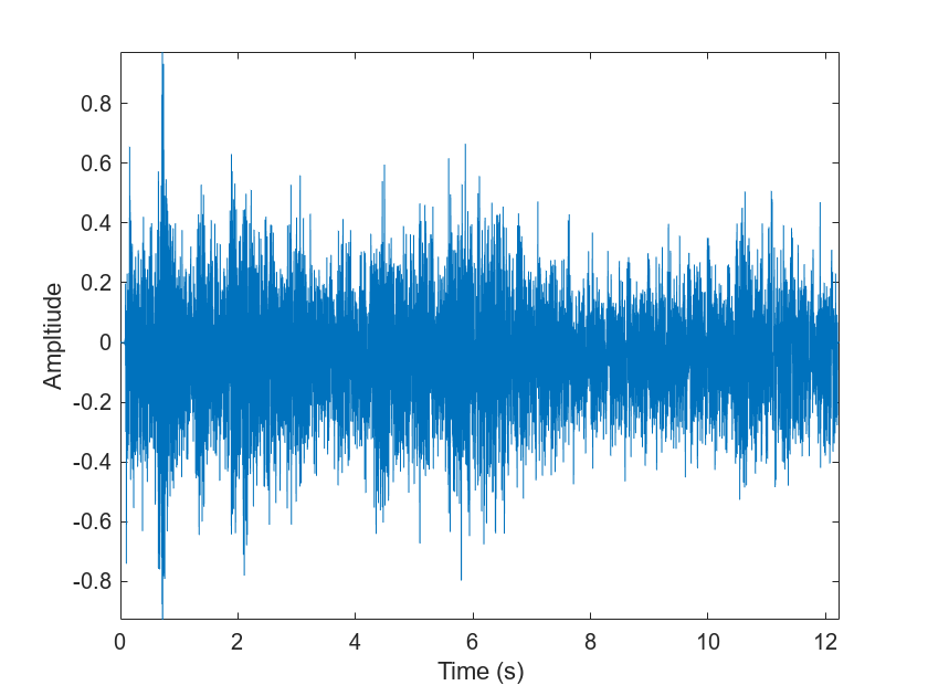
Read in an audio signal to extract feature embeddings from it.

[audioIn,fs] = audioread("Ambiance-16-44p1-mono-12secs.wav");

Plot and listen to the audio signal.

t = (0:numel(audioIn)-1)/fs;
plot(t,audioIn)
xlabel("Time (s)")
ylabel("Ampltiude")
axis tight

Figure contains an axes object. The axes object with xlabel Time (s), ylabel Ampltiude contains an object of type line.

sound(audioIn,fs)

VGGish requires you to preprocess the audio signal to match the input format used to train the network. The preprocesssing steps include resampling the audio signal and computing an array of mel spectrograms. To learn more about mel spectrograms, see melSpectrogram. Use vggishPreprocess to preprocess the signal and extract the mel spectrograms to be passed to VGGish. Visualize one of these spectrograms chosen at random.

spectrograms = vggishPreprocess(audioIn,fs);

arbitrarySpect = spectrograms(:,:,1,randi(size(spectrograms,4)));
surf(arbitrarySpect,EdgeColor="none")
view(90,-90)
xlabel("Mel Band")
ylabel("Frame")
title("Mel Spectrogram for VGGish")
axis tight

Figure contains an axes object. The axes object with title Mel Spectrogram for VGGish, xlabel Mel Band, ylabel Frame contains an object of type surface.

Create a VGGish neural network using the audioPretrainedNetwork function.

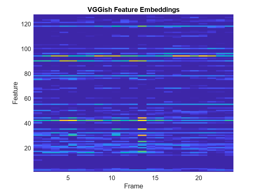
net = audioPretrainedNetwork("vggish");

Call predict with the network on the preprocessed mel spectrogram images to extract feature embeddings. The feature embeddings are returned as a numFrames-by-128 matrix, where numFrames is the number of individual spectrograms and 128 is the number of elements in each feature vector.

features = predict(net,spectrograms);
[numFrames,numFeatures] = size(features)

numFrames = 24

numFeatures = 128

Visualize the VGGish feature embeddings.

surf(features,EdgeColor="none")
view([90 -90])
xlabel("Feature")
ylabel("Frame")
title("VGGish Feature Embeddings")
axis tight

Figure contains an axes object. The axes object with title VGGish Feature Embeddings, xlabel Feature, ylabel Frame contains an object of type surface.

Transfer Learning Using VGGish

This example uses:

Open Live Script

In this example, you transfer the learning in the VGGish regression model to an audio classification task.

Download and unzip the environmental sound classification data set. This data set consists of recordings labeled as one of 10 different audio sound classes (ESC-10).

downloadFolder = matlab.internal.examples.downloadSupportFile("audio","ESC-10.zip");
unzip(downloadFolder,tempdir)
dataLocation = fullfile(tempdir,"ESC-10");

Create an audioDatastore object to manage the data and split it into train and validation sets. Call countEachLabel to display the distribution of sound classes and the number of unique labels.

ads = audioDatastore(dataLocation,IncludeSubfolders=true,LabelSource="foldernames");
labelTable = countEachLabel(ads)

labelTable=10×2 table
        Label         Count
    ______________    _____

    chainsaw           40  
    clock_tick         40  
    crackling_fire     40  
    crying_baby        40  
    dog                40  
    helicopter         40  
    rain               40  
    rooster            38  
    sea_waves          40  
    sneezing           40

Determine the total number of classes and their names.

numClasses = height(labelTable);
classNames = unique(ads.Labels);

Call splitEachLabel to split the data set into train and validation sets. Inspect the distribution of labels in the training and validation sets.

[adsTrain, adsValidation] = splitEachLabel(ads,0.8);

countEachLabel(adsTrain)

ans=10×2 table
        Label         Count
    ______________    _____

    chainsaw           32  
    clock_tick         32  
    crackling_fire     32  
    crying_baby        32  
    dog                32  
    helicopter         32  
    rain               32  
    rooster            30  
    sea_waves          32  
    sneezing           32

countEachLabel(adsValidation)

ans=10×2 table
        Label         Count
    ______________    _____

    chainsaw            8  
    clock_tick          8  
    crackling_fire      8  
    crying_baby         8  
    dog                 8  
    helicopter          8  
    rain                8  
    rooster             8  
    sea_waves           8  
    sneezing            8

The VGGish network expects audio to be preprocessed into log mel spectrograms. Use vggishPreprocess to extract the spectrograms from the train set. There are multiple spectrograms for each audio signal. Replicate the labels so that they are in one-to-one correspondence with the spectrograms.

overlapPercentage = 75;

trainFeatures = [];
trainLabels = [];
while hasdata(adsTrain)
    [audioIn,fileInfo] = read(adsTrain);
    features = vggishPreprocess(audioIn,fileInfo.SampleRate,OverlapPercentage=overlapPercentage);
    numSpectrograms = size(features,4);
    trainFeatures = cat(4,trainFeatures,features);
    trainLabels = cat(2,trainLabels,repelem(fileInfo.Label,numSpectrograms));
end

Extract spectrograms from the validation set and replicate the labels.

validationFeatures = [];
validationLabels = [];
segmentsPerFile = zeros(numel(adsValidation.Files), 1);
idx = 1;
while hasdata(adsValidation)
    [audioIn,fileInfo] = read(adsValidation);
    features = vggishPreprocess(audioIn,fileInfo.SampleRate,OverlapPercentage=overlapPercentage);
    numSpectrograms = size(features,4);
    validationFeatures = cat(4,validationFeatures,features);
    validationLabels = cat(2,validationLabels,repelem(fileInfo.Label,numSpectrograms));

    segmentsPerFile(idx) = numSpectrograms;
    idx = idx + 1;
end

Load the VGGish model and using audioPretrainedNetwork.

net = audioPretrainedNetwork("vggish");

Use addLayers (Deep Learning Toolbox) to add a fullyConnectedLayer (Deep Learning Toolbox) and a softmaxLayer (Deep Learning Toolbox) to the network. Set the WeightLearnRateFactor and BiasLearnRateFactor of the new fully connected layer to 10 so that learning is faster in the new layer than in the transferred layers.

net = addLayers(net,[ ...
    fullyConnectedLayer(numClasses,Name="FCFinal",WeightLearnRateFactor=10,BiasLearnRateFactor=10)
    softmaxLayer(Name="softmax")]);

Use connectLayers (Deep Learning Toolbox) to append the fully connected and softmax layers to the network.

net = connectLayers(net,"EmbeddingBatch","FCFinal");

To define training options, use trainingOptions (Deep Learning Toolbox).

miniBatchSize = 128;
options = trainingOptions("adam", ...
    MaxEpochs=5, ...
    MiniBatchSize=miniBatchSize, ...
    Shuffle="every-epoch", ...
    ValidationData={validationFeatures,validationLabels'}, ...
    ValidationFrequency=50, ...
    LearnRateSchedule="piecewise", ...
    LearnRateDropFactor=0.5, ...
    LearnRateDropPeriod=2, ...
    OutputNetwork="best-validation-loss", ...
    Verbose=false, ...
    Plots="training-progress",...
    Metrics="accuracy");

To train the network, use trainnet.

[trainedNet,netInfo] = trainnet(trainFeatures,trainLabels',net,"crossentropy",options);

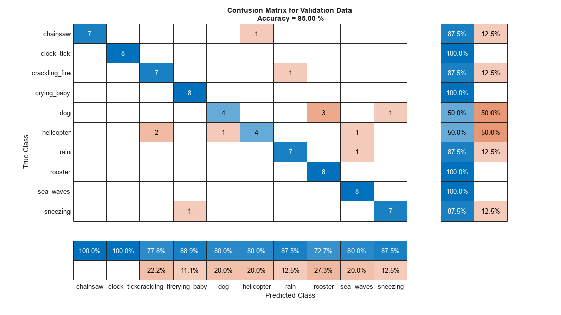
Each audio file was split into several segments to feed into the VGGish network. Combine the predictions for each file in the validation set using a majority-rule decision.

scores = predict(trainedNet,validationFeatures);
validationPredictions = scores2label(scores,classNames);

idx = 1;
validationPredictionsPerFile = categorical;
for ii = 1:numel(adsValidation.Files)
    validationPredictionsPerFile(ii,1) = mode(validationPredictions(idx:idx+segmentsPerFile(ii)-1));
    idx = idx + segmentsPerFile(ii);
end

Use confusionchart (Deep Learning Toolbox) to evaluate the performance of the network on the validation set.

figure(Units="normalized",Position=[0.2 0.2 0.5 0.5]);
confusionchart(adsValidation.Labels,validationPredictionsPerFile, ...
    Title=sprintf("Confusion Matrix for Validation Data \nAccuracy = %0.2f %%",mean(validationPredictionsPerFile==adsValidation.Labels)*100), ...
    ColumnSummary="column-normalized", ...
    RowSummary="row-normalized")

MATLAB figure

Visualize Mel Spectrogram for VGGish Input

Open Live Script

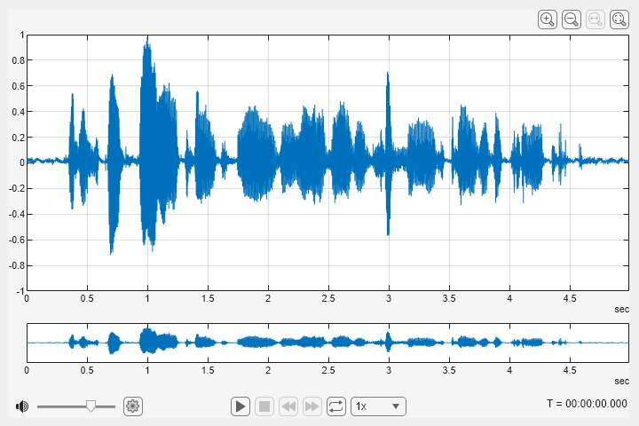
Read in an audio signal

[audioIn,fs] = audioread("SpeechDFT-16-8-mono-5secs.wav");

Use audioViewer to visualize and listen to the audio.

audioViewer(audioIn,fs)

Figure Audio Viewer contains an object of type uiaudioplayer.

Use vggishPreprocess to generate mel spectrograms that can be fed to the VGGish pretrained network. Specify additional outputs to get the center frequencies of the bands and the locations of the windows in time.

[spectrograms,cf,ts] = vggishPreprocess(audioIn,fs);

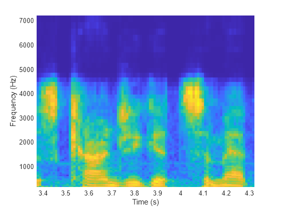
Choose a random spectrogram from the input to visualize. Use the center frequency and time location information to label the axes.

spectIdx = randi(size(spectrograms,4));
randSpect = spectrograms(:,:,1,spectIdx);
surf(cf,ts(:,spectIdx),randSpect,EdgeColor="none")
view([90 -90])
xlabel("Frequency (Hz)")
ylabel("Time (s)")
axis tight

Figure contains an axes object. The axes object with xlabel Frequency (Hz), ylabel Time (s) contains an object of type surface.

Input Arguments

collapse all

`audioIn` — Input signal
column vector | matrix

Input signal, specified as a column vector or matrix. If you specify a matrix, vggishPreprocess treats the columns of the matrix as individual audio channels.

Data Types: single | double

`fs` — Sample rate (Hz)
positive scalar

Sample rate of the input signal in Hz, specified as a positive scalar.

Data Types: single | double

`OP` — Overlap percentage between consecutive mel spectrograms
`50` (default) | scalar in the range [0,100)

Percentage overlap between consecutive mel spectrograms, specified as a scalar in the range [0,100).

Data Types: single | double

Output Arguments

collapse all

`features` — Mel spectrograms that can be fed to the VGGish pretrained network
`96`-by-`64`-by-`1`-by-K array

Mel spectrograms generated from audioIn, returned as a 96-by-64-by-1-by-K array, where:

96 –– Represents the number of 25 ms frames in each mel spectrogram.
64 –– Represents the number of mel bands spanning 125 Hz to 7.5 kHz.
K –– Represents the number of mel spectrograms and depends on the length of audioIn, the number of channels in audioIn, as well as OverlapPercentage.
Note
Each 96-by-64-by-1 patch represents a single mel spectrogram image. For multichannel inputs, mel spectrograms are stacked along the 4th dimension.

Data Types: single

`cf` — Center frequencies of mel bandpass filters
row vector

Center frequencies of the mel bandpass filters in Hz, returned as a row vector with length 64.

`ts` — Time location of each window
96-by-K matrix

Time location of the center of each analysis window of audio in seconds, returned as a 96-by-K matrix where K corresponds to the number of spectrograms in features. For multichannel inputs, the time stamps are stacked along the second dimension.

References

[1] Gemmeke, Jort F., et al. “Audio Set: An Ontology and Human-Labeled Dataset for Audio Events.” 2017 IEEE International Conference on Acoustics, Speech and Signal Processing (ICASSP), IEEE, 2017, pp. 776–80. DOI.org (Crossref),doi:10.1109/ICASSP.2017.7952261.

[2] Hershey, Shawn, et al. “CNN Architectures for Large-Scale Audio Classification.” 2017 IEEE International Conference on Acoustics, Speech and Signal Processing (ICASSP), IEEE, 2017, pp. 131–35. DOI.org (Crossref), doi:10.1109/ICASSP.2017.7952132.

Extended Capabilities

C/C++ Code Generation
Generate C and C++ code using MATLAB® Coder™.

GPU Arrays
Accelerate code by running on a graphics processing unit (GPU) using Parallel Computing Toolbox™.

This function fully supports GPU arrays. For more information, see Run MATLAB Functions on a GPU (Parallel Computing Toolbox).

Version History

Introduced in R2021a

expand all

R2024b: Additional outputs for center frequencies of bands and locations of windows in time

Call vggishPreprocess with additional output arguments to get the center frequencies of the bands and the time locations of the windows in the generated spectrograms.

vggishPreprocess

Syntax

Description

Examples

Extract Feature Embeddings Using VGGish

Transfer Learning Using VGGish

Visualize Mel Spectrogram for VGGish Input

Input Arguments

`audioIn` — Input signal
column vector | matrix

`fs` — Sample rate (Hz)
positive scalar

`OP` — Overlap percentage between consecutive mel spectrograms
`50` (default) | scalar in the range [0,100)

Output Arguments

`features` — Mel spectrograms that can be fed to the VGGish pretrained network
`96`-by-`64`-by-`1`-by-K array

`cf` — Center frequencies of mel bandpass filters
row vector

`ts` — Time location of each window
96-by-K matrix

References

Extended Capabilities

C/C++ Code Generation
Generate C and C++ code using MATLAB® Coder™.

GPU Arrays
Accelerate code by running on a graphics processing unit (GPU) using Parallel Computing Toolbox™.

Version History

R2024b: Additional outputs for center frequencies of bands and locations of windows in time

See Also

Apps

Blocks

Functions

vggishPreprocess

Syntax

Description

Examples

Extract Feature Embeddings Using VGGish

Transfer Learning Using VGGish

Visualize Mel Spectrogram for VGGish Input

Input Arguments

audioIn — Input signal column vector | matrix

fs — Sample rate (Hz) positive scalar

OP — Overlap percentage between consecutive mel spectrograms 50 (default) | scalar in the range [0,100)

Output Arguments

features — Mel spectrograms that can be fed to the VGGish pretrained network 96-by-64-by-1-by-K array

cf — Center frequencies of mel bandpass filters row vector

ts — Time location of each window 96-by-K matrix

References

Extended Capabilities

C/C++ Code Generation Generate C and C++ code using MATLAB® Coder™.

GPU Arrays Accelerate code by running on a graphics processing unit (GPU) using Parallel Computing Toolbox™.

Version History

R2024b: Additional outputs for center frequencies of bands and locations of windows in time

See Also

Apps

Blocks

Functions

`audioIn` — Input signal
column vector | matrix

`fs` — Sample rate (Hz)
positive scalar

`OP` — Overlap percentage between consecutive mel spectrograms
`50` (default) | scalar in the range [0,100)

`features` — Mel spectrograms that can be fed to the VGGish pretrained network
`96`-by-`64`-by-`1`-by-K array

`cf` — Center frequencies of mel bandpass filters
row vector

`ts` — Time location of each window
96-by-K matrix

C/C++ Code Generation
Generate C and C++ code using MATLAB® Coder™.

GPU Arrays
Accelerate code by running on a graphics processing unit (GPU) using Parallel Computing Toolbox™.