passiveplot

R2026b

Plot passivity index as function of frequency

collapse all in page

Syntax

passiveplot(G)

passiveplot(G1,G2,...,GN,___)

passiveplot(G1,LineSpec1,...,GN,LineSpecN)

passiveplot(___,type)

passiveplot(___,w)

passiveplot(___,plotoptions)

passiveplot(___,type,w,plotoptions)

passiveplot(___,Name=Value)

passiveplot(parent,___)

pp = passiveplot(___)

Description

The passiveplot function plots the passivity indices of a dynamic system model. To customize the plot, you can return a PassivePlot object and modify it using dot notation. For more information, see Customize Linear Analysis Plots at Command Line.

To obtain sector indices, use the passive function.

passiveplot(G) plots the relative passivity indices of the dynamic system G as a function of frequency. When I + G is minimum phase, the relative passivity indices are the singular values of (I - G)(I + G)^-1. The largest singular value measures the relative excess (R < 1) or shortage (R > 1) at each frequency. See getPassiveIndex for more information about the meaning of the passivity index.

passiveplot automatically chooses the frequency range and number of points for the plot based on the dynamics of G.

If G is a model with complex coefficients, then in:

Log frequency scale, the plot shows two branches, one for positive frequencies and one for negative frequencies. The arrows indicate the direction of increasing frequency values for each branch.
Linear frequency scale, the plot shows a single branch with a symmetric frequency range centered at a frequency value of zero.

example

passiveplot(G1,G2,...,GN,___) plots the passivity index for multiple dynamic systems G1,G2,...,GN on the same plot.

passiveplot(G1,LineSpec1,...,GN,LineSpecN) specifies a color, line style, and marker for each system in the plot.

example

passiveplot(___,type) plots the input, output, or I/O passivity index, depending on the specified type value.

You can use this syntax with any of the previous input-argument combinations.

example

passiveplot(___,w) plots the passivity index for frequencies specified by w. You can specify a frequency range or a vector of frequencies.

passiveplot(___,plotoptions) plots the passivity index with the plotting options specified in plotoptions. Settings you specify in plotoptions override the plotting preferences for the current MATLAB^® session. This syntax is useful when you want to write a script to generate multiple plots that look the same regardless of the local preferences.

example

passiveplot(___,type,w,plotoptions) plots the passivity index for any combination of type, w, and plotoptions in any order.

You can use this syntax with any of the previous input-argument combinations.

passiveplot(___,Name=Value) specifies response properties using one or more name-value arguments. For example, passiveplot(sys,Color="r") sets the plot color to red. (since R2026b)

When plotting responses for multiple systems, the specified name-value arguments apply to all responses.
The following name-value arguments override values specified in other input arguments.
- Frequency — Overrides frequencies specified using w
- PassiveType — Overrides passivity type specified using type
- Color — Overrides colors specified using LineSpec
- MarkerStyle — Overrides marker styles specified using LineSpec
- LineStyle — Overrides line styles specified using LineSpec

passiveplot(parent,___) plots the passivity indices in the specified parent graphics container, such as a Figure or TiledChartLayout, and sets the Parent property. Use this syntax when you want to create a plot in a specified open figure or when creating apps in App Designer. (since R2026b)

pp = passiveplot(___) plots the passivity indices and returns the corresponding chart object. To customize the appearance and behavior of the response plot, modify the chart object properties using dot notation. (since R2026b)

Examples

collapse all

Plot Passivity Versus Frequency

Open Live Script

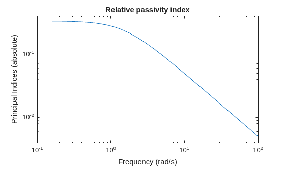
Plot the relative passivity index as a function of frequency of the system $G = (s + 2) / (s + 1)$ .

G = tf([1 2],[1 1]); 
passiveplot(G)

MATLAB figure

The plot shows that the relative passivity index is less than 1 at all frequencies. Therefore, the system G is passive.

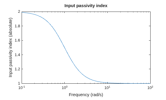
Plot the input passivity index of the same system.

passiveplot(G,"input")

MATLAB figure

The input passivity index is positive at all frequencies. Therefore, the system is input strictly passive.

Plot Passivity of Multiple Systems

Open Live Script

Plot the input passivity index of two dynamic systems and their series interconnection.

G1 = tf([5 3 1],[1 2 1]);
G2 = tf([1 1 5 0.1],[1 2 3 4]);
H = G2*G1;

passiveplot(G1,"r",G2,"b--",H,"gx","input")

legend("G1","G2","G2*G1");

The input passivity index of the interconnected system dips below 0 around 1 rad/s. This plot shows that the series interconnection of two passive systems is not necessarily passive. However, passivity is preserved for parallel or feedback interconnections of passive systems.

Plot Passivity of Models with Complex Coefficients

Open Live Script

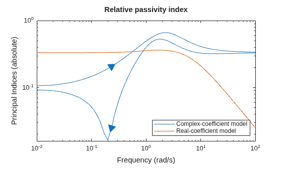
Plot the relative passivity indices of a complex-coefficient model and a real-coefficient model on the same plot.

A = [-3.50,-1.25-0.25i;2,0];
B = [1;0];
C = [-0.75-0.5i,0.625-0.125i];
D = 0.5;
Gc = ss(A,B,C,D);
Gr = tf([1 5 10],[1 10 5]);
passiveplot(Gc,Gr)
legend("Complex-coefficient model","Real-coefficient model", ...
    Location="southeast");

In log frequency scale, the plot shows two branches for models with complex coefficients, one for positive frequencies, with a right-pointing arrow, and one for negative frequencies, with a left-pointing arrow. In both branches, the arrows indicate the direction of increasing frequencies. The plots for models with real coefficients always contain a single branch with no arrows.

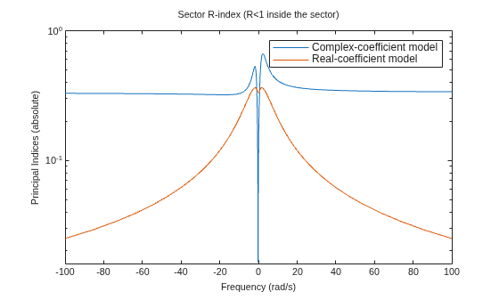
Set the plotting frequency scale to linear.

opt = sectorplotoptions;
opt.FreqScale = "Linear";

Plot the indices.

passiveplot(Gc,Gr,opt)

MATLAB figure

legend("Complex-coefficient model","Real-coefficient model");

MATLAB figure

In linear frequency scale, the plots show a single branch with a symmetric frequency range centered at a frequency value of zero. The plot also shows the negative-frequency response of a real-coefficient model when you plot the response along with a complex-coefficient model.

Input Arguments

collapse all

`G` — Model to analyze
dynamic system model | model array

Model to analyze for passivity, specified as a dynamic system model such as a tf, ss, or genss model. G can be MIMO, if the number of inputs equals the number of outputs. G can be continuous or discrete. If G is a generalized model with tunable or uncertain blocks, passiveplot evaluates passivity of the current, nominal value of G.

If G is a model array, then passiveplot plots the passivity index of all models in the array on the same plot. When you use output arguments to get passivity data, G must be a single model.

`type` — Type of passivity index
`"input"` | `"output"` | `"io"'`

Type of passivity index, specified as one of the following:

"input" — Input passivity index (input feedforward passivity). This value is the smallest eigenvalue of $(G (s) + G {(s)}^{H}) / 2$ , for s = jω in continuous time, and s = e_jω in discrete time.
"output" — Output passivity index (output feedback passivity). When G is minimum phase, this value is the smallest eigenvalue of $(G {(s)}^{- 1} + G {(s)}^{- H}) / 2$ , for s = jω in continuous time, and s = e_jω in discrete time.
"io" — Combined I/O passivity index. When I + G is minimum phase, this value is the largest τ(ω) such that:
$G (s) + G {(s)}^{H} > 2 τ (ω) (I + G {(s)}^{H} G (s)),$
for s = jω in continuous time, and s = e_jω in discrete time.

See About Passivity and Passivity Indices for details about these indices.

`w` — Frequencies
`{wmin,wmax}` | vector

Frequencies at which to compute and plot indices, specified as one of the following:

Cell array of the form {wmin,wmax} — Compute the plot indices at frequencies in the range from wmin to wmax. If wmax is greater than the Nyquist frequency of the system, the response is computed only up to the Nyquist frequency.
Vector of frequencies — Compute the plot indices at each specified frequency. For example, use logspace to generate a row vector with logarithmically spaced frequency values. The vector w can contain both positive and negative frequencies.
[] — Automatically select frequencies based on system dynamics.

For models with complex coefficients, if you specify a frequency range of [w_min,w_max] for your plot, then in:

Log frequency scale, the plot frequency limits are set to [w_min,w_max] and the plot shows two branches, one for positive frequencies [w_min,w_max] and one for negative frequencies [–w_max,–w_min].
Linear frequency scale, the plot frequency limits are set to [–w_max,w_max] and the plot shows a single branch with a symmetric frequency range centered at a frequency value of zero.

Specify frequencies in units of rad/TimeUnit, where TimeUnit is the TimeUnit property of the model.

`LineSpec` — Line style, marker, and color
string | character vector

Line style, marker, and color, specified as a string or character vector containing symbols. The symbols can appear in any order. You do not need to specify all three characteristics. For example, specify the marker and omit the line style, then the plot shows only the marker and no line.

Example: '--or' is a red dashed line with circle markers.

Line Style	Description
`"-"`	Solid line
`"--"`	Dashed line
`":"`	Dotted line
`"-."`	Dash-dotted line

Marker	Description
`"o"`	Circle
`"+"`	Plus sign
`"*"`	Asterisk
`"."`	Point
`"x"`	Cross
`"_"`	Horizontal line
`"\|"`	Vertical line
`"s"`	Square
`"d"`	Diamond
`"^"`	Upward-pointing triangle
`"v"`	Downward-pointing triangle
`">"`	Right-pointing triangle
`"<"`	Left-pointing triangle
`"p"`	Pentagram
`"h"`	Hexagram

Color	Description
`"r"`	red
`"g"`	green
`"b"`	blue
`"c"`	cyan
`"m"`	magenta
`"y"`	yellow
`"k"`	black
`"w"`	white

`plotoptions` — Passivity index plot options
`SectorPlotOptions` object

Passivity index plot options, specified as a SectorPlotOptions object created using sectorplotoptions. You can use these options to customize the plot appearance. Settings you specify in plotoptions override the preference settings for the current MATLAB session.

`parent` — Parent graphics container
`Figure` object | `TiledChartLayout` object | `UIFigure` object | `UIGridLayout` object | `UIPanel` object | `UITab` object

Parent graphics container, specified as one of these objects:

Figure
TiledChartLayout
UIFigure
UIGridLayout
UIPanel
UITab

Name-Value Arguments

collapse all

Specify optional pairs of arguments as Name1=Value1,...,NameN=ValueN, where Name is the argument name and Value is the corresponding value. Name-value arguments must appear after other arguments, but the order of the pairs does not matter.

Example: passiveplot(sys,LegendDisplay="off") hides the response of sys from the plot legend.

`Frequency` — Frequencies
`{wmin,wmax}` | vector

Frequencies at which to compute and plot indices, specified as one of the following:

Cell array of the form {wmin,wmax} — Compute the plot indices at frequencies in the range from wmin to wmax. If wmax is greater than the Nyquist frequency of the system, the response is computed only up to the Nyquist frequency.
Vector of frequencies — Compute the plot indices at each specified frequency. For example, use logspace to generate a row vector with logarithmically spaced frequency values. The vector can contain both positive and negative frequencies.
[] — Automatically select frequencies based on system dynamics.

For models with complex coefficients, if you specify a frequency range of [w_min,w_max] for your plot, then in:

Log frequency scale, the plot frequency limits are set to [w_min,w_max] and the plot shows two branches, one for positive frequencies [w_min,w_max] and one for negative frequencies [–w_max,–w_min].
Linear frequency scale, the plot frequency limits are set to [–w_max,w_max] and the plot shows a single branch with a symmetric frequency range centered at a frequency value of zero.

Specify frequencies in units of rad/TimeUnit, where TimeUnit is the TimeUnit property of the model.

`PassiveType` — Type of passivity index
`"input"` | `"output"` | `"io"'`

Type of passivity index, specified as one of the following:

"input" — Input passivity index (input feedforward passivity). This value is the smallest eigenvalue of $(G (s) + G {(s)}^{H}) / 2$ , for s = jω in continuous time, and s = e_jω in discrete time.
"output" — Output passivity index (output feedback passivity). When G is minimum phase, this value is the smallest eigenvalue of $(G {(s)}^{- 1} + G {(s)}^{- H}) / 2$ , for s = jω in continuous time, and s = e_jω in discrete time.
"io" — Combined I/O passivity index. When I + G is minimum phase, this value is the largest τ(ω) such that:
$G (s) + G {(s)}^{H} > 2 τ (ω) (I + G {(s)}^{H} G (s)),$
for s = jω in continuous time, and s = e_jω in discrete time.

See About Passivity and Passivity Indices for details about these indices.

`Name` — Response name
string | character vector

Response name, specified as a string or character vector and stored as a string.

`Visible` — Response visibility
`"on"` (default) | on/off logical value

Response visibility, specified as one of these logical on/off values:

"on", 1, or true — Display the response in the plot.
"off", 0, or false — Do not display the response in the plot.

The value is stored as an on/off logical value of type matlab.lang.OnOffSwitchState.

`LegendDisplay` — Option to list response in legend
`"on"` (default) | on/off logical value

Option to list the response in the legend, specified as one of these logical on/off values:

"on", 1, or true — List the response in the legend.
"off", 0, or false — Do not list the response in the legend.

The value is stored as an on/off logical value of type matlab.lang.OnOffSwitchState.

`MarkerStyle` — Marker style
`"none"` | `"o"` | `"+"` | `"*"` | `"."` | ...

Marker style, specified as one of these values. Specifying a marker style using a name-value argument overrides any marker style that you specify using LineSpec.

Marker	Description
`"none"`	No marker
`"o"`	Circle
`"+"`	Plus sign
`"*"`	Asterisk
`"."`	Point
`"x"`	Cross
`"_"`	Horizontal line
`"\|"`	Vertical line
`"s"`	Square
`"d"`	Diamond
`"^"`	Upward-pointing triangle
`"v"`	Downward-pointing triangle
`">"`	Right-pointing triangle
`"<"`	Left-pointing triangle
`"p"`	Pentagram
`"h"`	Hexagram

`Color` — Plot color
RGB triplet | hexadecimal color code | color name

Plot color, specified as an RGB triplet or a hexadecimal color code and stored as an RGB triplet. Specifying a color using a name-value argument overrides any color that you specify using LineSpec.

You can also specify some common colors by name. This table lists these colors and their corresponding RGB triplets and hexadecimal color codes.

Color Name	RGB Triplet	Hexadecimal Color Code
`"red"` or `"r"`	`[1 0 0]`	`#FF0000`
`"green"` or `"g"`	`[0 1 0]`	`#00FF00`
`"blue"` or `"b"`	`[0 0 1]`	`#0000FF`
`"cyan"` or `"c"`	`[0 1 1]`	`#00FFFF`
`"magenta"` or `"m"`	`[1 0 1]`	`#FF00FF`
`"yellow"` or `"y"`	`[1 1 0]`	`#FFFF00`
`"black"` or `"k"`	`[0 0 0]`	`#000000`
`"white"` or `"w"`	`[1 1 1]`	`#FFFFFF`

`LineStyle` — Line style
`"-"` | `"--"` | `":"` | `"-."`

Line style, specified as one of these values. Specifying a line style using a name-value argument overrides any line style that you specify using LineSpec.

Line Style	Description
`"-"`	Solid line
`"--"`	Dashed line
`":"`	Dotted line
`"-."`	Dash-dotted line
`"none"`	No line

`MarkerSize` — Marker size
positive scalar

Marker size, specified as a positive scalar.

`LineWidth` — Line width
positive scalar

Line width, specified as a positive scalar.

`SeriesIndex` — Series index
positive integer | `"none"`

Series index, specified as a positive integer or "none".

By default, the SeriesIndex property is a number that corresponds to the order in which the response was added to the chart, starting at 1. MATLAB uses the number to calculate indices for automatically assigning color, line style, or markers for responses. Any responses in the chart that have the same SeriesIndex number also have the same color, line style, and markers.

A SeriesIndex value of "none" indicates that a response does not participate in the indexing scheme.

Output Arguments

collapse all

`pp` — Chart object
`PassivePlot` object

Chart object, returned as a PassivePlot object. To customize your plot appearance and behavior, modify the properties of this object using dot notation. For more information, see PassivePlot Properties.

Version History

Introduced in R2016a

expand all

R2026b: Improved customization workflows and integration with MATLAB plotting tools

Starting in R2026b, the passiveplot function returns a PassivePlot chart object.

Previously, the passiveplot function returned the computed passivity indices. To obtain computed passivity indices, use the new passive function. For more information, see Obtain passivity indices using passive function.

The new chart object allows you to customize your plot using dot notation and name-value arguments.

The new chart object also improves integration with MATLAB plotting tools. For example:

You can now add passivity plots to tiled chart layouts.
Saving and loading a parent figure now maintains full plot interactivity.
You can add a response to your passivity plot using the addResponse function.

R2026b: Obtain passivity indices using `passive` function

Starting in R2026b, you obtain computed passivity indices using the new passive function instead of the passiveplot function.

For these computation workflows, only the name of the plotting function has changed. The computation behavior remains the same.

passiveplot

Syntax

Description

Examples

Plot Passivity Versus Frequency

Plot Passivity of Multiple Systems

Plot Passivity of Models with Complex Coefficients

Input Arguments

`G` — Model to analyze
dynamic system model | model array

`type` — Type of passivity index
`"input"` | `"output"` | `"io"'`

`w` — Frequencies
`{wmin,wmax}` | vector

`LineSpec` — Line style, marker, and color
string | character vector

`plotoptions` — Passivity index plot options
`SectorPlotOptions` object

`parent` — Parent graphics container
`Figure` object | `TiledChartLayout` object | `UIFigure` object | `UIGridLayout` object | `UIPanel` object | `UITab` object

Name-Value Arguments

`Frequency` — Frequencies
`{wmin,wmax}` | vector

`PassiveType` — Type of passivity index
`"input"` | `"output"` | `"io"'`

`Name` — Response name
string | character vector

`Visible` — Response visibility
`"on"` (default) | on/off logical value

`LegendDisplay` — Option to list response in legend
`"on"` (default) | on/off logical value

`MarkerStyle` — Marker style
`"none"` | `"o"` | `"+"` | `"*"` | `"."` | ...

`Color` — Plot color
RGB triplet | hexadecimal color code | color name

`LineStyle` — Line style
`"-"` | `"--"` | `":"` | `"-."`

`MarkerSize` — Marker size
positive scalar

`LineWidth` — Line width
positive scalar

`SeriesIndex` — Series index
positive integer | `"none"`

Output Arguments

`pp` — Chart object
`PassivePlot` object

Version History

R2026b: Improved customization workflows and integration with MATLAB plotting tools

R2026b: Obtain passivity indices using `passive` function

See Also

Topics

passiveplot

Syntax

Description

Examples

Plot Passivity Versus Frequency

Plot Passivity of Multiple Systems

Plot Passivity of Models with Complex Coefficients

Input Arguments

G — Model to analyze dynamic system model | model array

type — Type of passivity index "input" | "output" | "io"'

w — Frequencies {wmin,wmax} | vector

LineSpec — Line style, marker, and color string | character vector

plotoptions — Passivity index plot options SectorPlotOptions object

parent — Parent graphics container Figure object | TiledChartLayout object | UIFigure object | UIGridLayout object | UIPanel object | UITab object

Name-Value Arguments

Frequency — Frequencies {wmin,wmax} | vector

PassiveType — Type of passivity index "input" | "output" | "io"'

Name — Response name string | character vector

Visible — Response visibility "on" (default) | on/off logical value

LegendDisplay — Option to list response in legend "on" (default) | on/off logical value

MarkerStyle — Marker style "none" | "o" | "+" | "*" | "." | ...

Color — Plot color RGB triplet | hexadecimal color code | color name

LineStyle — Line style "-" | "--" | ":" | "-."

MarkerSize — Marker size positive scalar

LineWidth — Line width positive scalar

SeriesIndex — Series index positive integer | "none"

Output Arguments

pp — Chart object PassivePlot object

Version History

R2026b: Improved customization workflows and integration with MATLAB plotting tools

R2026b: Obtain passivity indices using passive function

See Also

Topics

`G` — Model to analyze
dynamic system model | model array

`type` — Type of passivity index
`"input"` | `"output"` | `"io"'`

`w` — Frequencies
`{wmin,wmax}` | vector

`LineSpec` — Line style, marker, and color
string | character vector

`plotoptions` — Passivity index plot options
`SectorPlotOptions` object

`parent` — Parent graphics container
`Figure` object | `TiledChartLayout` object | `UIFigure` object | `UIGridLayout` object | `UIPanel` object | `UITab` object

`Frequency` — Frequencies
`{wmin,wmax}` | vector

`PassiveType` — Type of passivity index
`"input"` | `"output"` | `"io"'`

`Name` — Response name
string | character vector

`Visible` — Response visibility
`"on"` (default) | on/off logical value

`LegendDisplay` — Option to list response in legend
`"on"` (default) | on/off logical value

`MarkerStyle` — Marker style
`"none"` | `"o"` | `"+"` | `"*"` | `"."` | ...

`Color` — Plot color
RGB triplet | hexadecimal color code | color name

`LineStyle` — Line style
`"-"` | `"--"` | `":"` | `"-."`

`MarkerSize` — Marker size
positive scalar

`LineWidth` — Line width
positive scalar

`SeriesIndex` — Series index
positive integer | `"none"`

`pp` — Chart object
`PassivePlot` object

R2026b: Obtain passivity indices using `passive` function