Closing Feedback Loops with Time Delays
This example shows how internal delays arise when you interconnect models that have input, output, or transport time delays.
Create a model of the following control architecture:

G is the plant model, which has an input
delay. C is a proportional-integral (PI) controller.
To create a model representing the closed-loop response of this system:
Create the plant
Gand the controllerC.G = tf(1,[1 10],'InputDelay',2.1); C = pid(0.5,2.3);Chas a proportional gain of 0.5 and an integral gain of 2.3.Use
feedbackto compute the closed-loop response from r to y.T = feedback(C*G,1);
The time delay in T is not an input delay
as it is in G. Because the time delay is internal
to the closed-loop system, the software returns T as
an ss model with an internal time
delay of 2.1 seconds.
Note
In addition to feedback,
any system interconnection function (including parallel and series)
can give rise to internal delays.
T is an exact representation of the closed-loop response, not an approximation. To access the internal delay value, enter:
T.InternalDelay
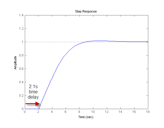
A step plot of T confirms the presence of the time delay:
step(T)

The internal time delay is stored in the InternalDelay property
of T. Use dot notation to access InternalDelay.
For example, to change the internal delay to 3.5 seconds, enter:
T.InternalDelay = 3.5
You cannot modify the number of internal delays because they are structural properties of the model.