differentiate

Differentiate cfit or sfit object

collapse all in page

Syntax

fx = differentiate(FO, X)

[fx, fxx] = differentiate(FO, X)

[fx, fy] = differentiate(FO, X, Y)

[fx, fy] = differentiate(FO, [X, Y])

[fx, fy, fxx, fxy, fyy] = differentiate(FO, ...)

Description

Note

Use these syntaxes for cfit objects.

fx = differentiate(FO, X) differentiates the cfit object FO at the points specified by the vector X and returns the result in fx.

[fx, fxx] = differentiate(FO, X) differentiates the cfit object FO at the points specified by the vector X and returns the result in fx and the second derivative in fxx.

example

Note

Use these syntaxes for sfit objects.

[fx, fy] = differentiate(FO, X, Y) differentiates the surface FO at the points specified by X and Y and returns the result in fx and fy.

FO is a surface fit (sfit) object generated by the fit function.

X and Y must be double-precision arrays and the same size and shape as each other.

All return arguments are the same size and shape as X and Y.

If FO represents the surface $z = f (x, y)$ , then FX contains the derivatives with respect to x, that is, $\frac{d f}{d x}$ , and FY contains the derivatives with respect to y, that is, $\frac{d f}{d y}$ .

[fx, fy] = differentiate(FO, [X, Y]), where X and Y are column vectors, allows you to specify the evaluation points as a single argument.

[fx, fy, fxx, fxy, fyy] = differentiate(FO, ...) computes the first and second derivatives of the surface fit object FO.

fxx contains the second derivatives with respect to x, that is, $\frac{\partial^{2} f}{\partial x^{2}}$ .

fxy contains the mixed second derivatives, that is, $\frac{\partial^{2} f}{\partial x \partial y}$ .

fyy contains the second derivatives with respect to y, that is, $\frac{\partial^{2} f}{\partial y^{2}}$ .

Examples

collapse all

Find the Derivatives of a Curve Using the `differentiate` Function

Open Live Script

Create a baseline sinusoidal signal.

xdata = (0:.1:2*pi)';
y0 = sin(xdata);

Add response-dependent Gaussian noise to the signal.

noise = 2*y0.*randn(size(y0)); 											
ydata = y0 + noise;

Fit the noisy data with a custom sinusoidal model.

f = fittype('a*sin(b*x)');
fit1 = fit(xdata,ydata,f,'StartPoint',[1 1]);

Find the derivatives of the fit at the predictors.

[d1,d2] = differentiate(fit1,xdata);

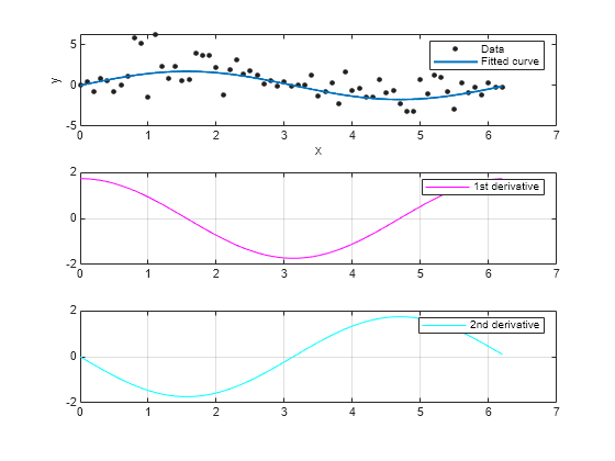
Plot the data, the fit, and the derivatives.

subplot(3,1,1)
plot(fit1,xdata,ydata) % cfit plot method
subplot(3,1,2)
plot(xdata,d1,'m') % double plot method
grid on
legend('1st derivative')
subplot(3,1,3)
plot(xdata,d2,'c') % double plot method
grid on
legend('2nd derivative')

Figure contains 3 axes objects. Axes object 1 with xlabel x, ylabel y contains 2 objects of type line. One or more of the lines displays its values using only markers These objects represent Data, Fitted curve. Axes object 2 contains an object of type line. This object represents 1st derivative. Axes object 3 contains an object of type line. This object represents 2nd derivative.

You can also compute and plot derivatives directly with the cfit plot method, as follows:

figure
plot(fit1,xdata,ydata,{'fit','deriv1','deriv2'})

The plot method, however, does not return data on the derivatives, unlike the differentiate method.

Find the Derivatives of a Surface Using the `differentiate` Function

Open Live Script

You can use the differentiate method to compute the gradients of a fit and then use the quiver function to plot these gradients as arrows. This example plots the gradients over the top of a contour plot.

Create the derivation points and fit the data.

x = [0.64;0.95;0.21;0.71;0.24;0.12;0.61;0.45;0.46;...
0.66;0.77;0.35;0.66];
y = [0.42;0.84;0.83;0.26;0.61;0.58;0.54;0.87;0.26;...
0.32;0.12;0.94;0.65];
z = [0.49;0.051;0.27;0.59;0.35;0.41;0.3;0.084;0.6;...
0.58;0.37;0.19;0.19];
fo = fit( [x, y], z, 'poly32', 'normalize', 'on' );
[xx, yy] = meshgrid( 0:0.04:1, 0:0.05:1 );

Compute the gradients of the fit using the differentiate function.

[fx, fy] = differentiate( fo, xx, yy );

Use the quiver function to plot the gradients.

plot( fo, 'Style', 'Contour' );
hold on
h = quiver( xx, yy, fx, fy, 'r', 'LineWidth', 2 );
hold off
colormap( copper )

Figure contains an axes object. The axes object contains 2 objects of type contour, quiver.

If you want to use derivatives in an optimization, you can, for example, implement an objective function for fmincon as follows.

function [z, g, H] = objectiveWithHessian( xy )

% The input xy represents a single evaluation point

z = f( xy );

if nargout > 1

[fx, fy, fxx, fxy, fyy] = differentiate( f, xy );

g = [fx, fy];

H = [fxx, fxy; fxy, fyy];

end

Input Arguments

collapse all

`FO` — `cfit` function
`cfit` | `sfit`

Function to differentiate, specified as a cfit object for curves or as a sfit object for surfaces.

`X` — Differentiation points
array

Points at which to differentiate the function, specified as a vector. For surfaces, this argument must have the same size and shape of Y.

`Y` — Differentiation points
array

Points at which to differentiate the function, specified as a vector. For surfaces, this argument must have the same size and shape of X.

Output Arguments

collapse all

`fx` — First derivative with respect to `x`
vector

First derivative of the function, returned as a vector of the same size and shape of X and Y.

If FO is a surface, $z = f (x, y)$ , then fx contains the derivatives with respect to x.

`fxx` — Second derivative with respect to `x`
vector

Second derivative of the function, returned as a vector of the same size and shape of X and Y.

If FO is a surface, $z = f (x, y)$ , then fxx contains the second derivatives with respect to x.

`fy` — First derivative with respect to `y`
vector

First derivative of the function, returned as a vector of the same size and shape of X and Y.

If FO is a surface, $z = f (x, y)$ , then fy contains the derivatives with respect to y.

`fyy` — Second derivative with respect to `y`
vector

Second derivative of the function, returned as a vector of the same size and shape of X and Y.

If FO is a surface, $z = f (x, y)$ , then fyy contains the second derivatives with respect to y.

`fxy` — Mixed second derivative
vector

Mixed second derivative of the function, returned as a vector of the same size and shape of X and Y.

Tips

For library models with closed forms, the toolbox calculates derivatives analytically. For all other models, the toolbox calculates the first derivative using the centered difference quotient

$\frac{d f}{d x} = \frac{f (x + Δ x) - f (x - Δ x)}{2 Δ x}$

where x is the value at which the toolbox calculates the derivative, $Δ x$ is a small number (on the order of the cube root of eps), $f (x + Δ x)$ is fun evaluated at $x + Δ x$ , and $f (x - x Δ)$ is fun evaluated at $x - Δ x$ .

The toolbox calculates the second derivative using the expression

$\frac{d^{2} f}{d x^{2}} = \frac{f (x + Δ x) + f (x - Δ x) - 2 f (x)}{{(Δ x)}^{2}}$

The toolbox calculates the mixed derivative for surfaces using the expression

$\frac{\partial^{2} f}{\partial x \partial y} (x, y) = \frac{f (x + Δ x, y + Δ y) - f (x - Δ x, y + Δ y) - f (x + Δ x, y - Δ y) + f (x - Δ x, y - Δ y)}{4 Δ x Δ y}$

Version History

Introduced before R2006a

differentiate

Syntax

Description

Examples

Find the Derivatives of a Curve Using the `differentiate` Function

Find the Derivatives of a Surface Using the `differentiate` Function

Input Arguments

`FO` — `cfit` function
`cfit` | `sfit`

`X` — Differentiation points
array

`Y` — Differentiation points
array

Output Arguments

`fx` — First derivative with respect to `x`
vector

`fxx` — Second derivative with respect to `x`
vector

`fy` — First derivative with respect to `y`
vector

`fyy` — Second derivative with respect to `y`
vector

`fxy` — Mixed second derivative
vector

Tips

Version History

See Also

Topics

differentiate

Syntax

Description

Examples

Find the Derivatives of a Curve Using the differentiate Function

Find the Derivatives of a Surface Using the differentiate Function

Input Arguments

FO — cfit function cfit | sfit

X — Differentiation points array

Y — Differentiation points array

Output Arguments

fx — First derivative with respect to x vector

fxx — Second derivative with respect to x vector

fy — First derivative with respect to y vector

fyy — Second derivative with respect to y vector

fxy — Mixed second derivative vector

Tips

Version History

See Also

Topics

Find the Derivatives of a Curve Using the `differentiate` Function

Find the Derivatives of a Surface Using the `differentiate` Function

`FO` — `cfit` function
`cfit` | `sfit`

`X` — Differentiation points
array

`Y` — Differentiation points
array

`fx` — First derivative with respect to `x`
vector

`fxx` — Second derivative with respect to `x`
vector

`fy` — First derivative with respect to `y`
vector

`fyy` — Second derivative with respect to `y`
vector

`fxy` — Mixed second derivative
vector