Custom Models

Custom Models vs. Library Models

If the Curve Fitting Toolbox™ library does not contain a desired parametric equation, you can create your own custom equation. Library models, however, offer the best chance for rapid convergence. This is because:

For most library models, the toolbox calculates optimal default coefficient starting points. For custom models, the toolbox chooses random default starting points on the interval [0,1]. You need to find suitable start points for custom models.
Library models use an analytic Jacobian. Custom models use finite differencing.

Linear and Nonlinear Fitting

You can create custom general equations with the Custom Equation fit type. General models are nonlinear combinations of (perhaps nonlinear) terms. They are defined by equations that might be nonlinear in the parameters. The custom equation fit uses the nonlinear least-squares fitting procedure.

You can define a custom linear equation using the Custom Equation fit type, though the nonlinear fitting is less efficient and usually slower than linear least-squares fitting.

If you don’t know if your equation can be expressed as a set of linear functions, then choose Custom Equation. You might need to search for suitable start points.
If you need linear least-squares fitting for custom equations, choose the Linear Fitting model type instead. See Custom Linear Fitting.

Selecting a Custom Equation Fit Interactively

In the Curve Fitter app, on the Curve Fitter tab, in the Fit Type section, click the arrow to open the gallery. In the fit gallery, click Custom Equation in the Custom group.

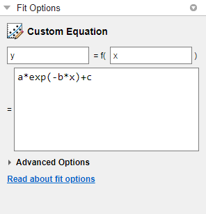
In the Fit Options pane, use the custom equation fit to define your own equations. An example custom equation appears when you click Custom Equation, as shown here for curve data.

Default custom equation for a curve fit

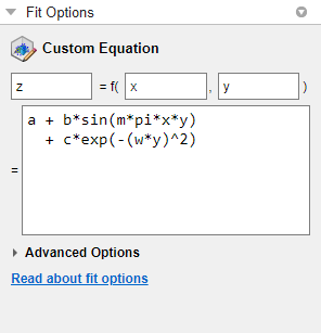
If you have surface data, the example custom equation uses both x and y.

Default custom equation for a surface fit

You can edit x, y, and z to any valid variable names.
In the lower box, edit the example to define your own custom equation. You can enter any valid MATLAB^® expression in terms of your variable names. You can specify a function or script name (see Fitting a Curve Defined by a File in the Curve Fitter App).
Click Advanced Options if you want to specify start points or bounds. By default, the starting values are randomly selected on the interval [0,1] and are unconstrained. You might need to search for suitable start points and bounds. For an example, see Custom Nonlinear ENSO Data Analysis.
If you set fit options and then alter other fit settings, the app remembers your choices for lower and upper bounds and start points, if possible. For custom equations, the Curve Fitter app always remembers user values. However, for many library models, if you change fit settings, then the app automatically calculates new best values for start points or lower bounds.

You can save your custom equations as part of your saved Curve Fitter app sessions.

Your function can execute a number of times, both during fitting and during preprocessing before fitting. Be aware this may be time-consuming if you are using functions with side effects such as writing data to a file, or displaying diagnostic information to the Command Window.

For examples, see:

Fitting a Curve Defined by a File in the Curve Fitter App

This example shows how to provide a function or script name as the fitting model in the Curve Fitter app. Define a function in a file and use it to fit a curve.

Define a function in a MATLAB file.

function y = piecewiseLine(x,a,b,c,d,k)
% PIECEWISELINE   A line made of two pieces
% that is not continuous.

y = zeros(size(x));

% This example includes a for-loop and if statement
% purely for example purposes.
for i = 1:length(x)
    if x(i) < k
        y(i) = a + b.* x(i);
    else
        y(i) = c + d.* x(i);
    end
end
end

Save the file on the MATLAB path.

Define some data and open the Curve Fitter app.

x = [0.81;0.91;0.13;0.91;0.63;0.098;0.28;0.55; ...
    0.96;0.96;0.16;0.97;0.96];
y = [0.17;0.12;0.16;0.0035;0.37;0.082;0.34;0.56; ...
    0.15;-0.046;0.17;-0.091;-0.071];

curveFitter

In the Curve Fitter app, on the Curve Fitter tab, in the Data section, click Select Data. In the Select Fitting Data dialog box, select x and y in the X data and Y data lists, respectively. Enter Piecewise Function as the fit name.
Use your piecewiseLine function in the Curve Fitter app. On the Curve Fitter tab, in the Fit Type section, click the arrow to open the gallery. In the fit gallery, click Custom Equation in the Custom group. In the Fit Options pane, enter your function expression in the custom equation text box. The function takes x data and some parameters for fitting.
```
piecewiseLine(x,a,b,c,d,k)
```
The Curve Fitter app creates a fit using your function.

Custom equation using piecewise line function

Tip

If you want to use the same function for fitting at the command line, use the same expression as an input to fittype, and then use the fittype as an input to fit:

ft = fittype("piecewiseLine(x,a,b,c,d,k)");
f = fit(x,y,ft)

For more examples, see the fit function.

Selecting a Custom Equation Fit at the Command Line

To fit custom models, either:

Supply a custom model to the fit function in the fitType input argument. You can use a MATLAB expression (including any .m file), a cell array or string array of linear model terms, or an anonymous function.
Create a fittype object with the fittype function to use as an input argument for the fit function.

This example loads some data and uses a custom equation defining a Weibull model as an input to the fit function:

time = [ 0.1;  0.1;  0.3;  0.3;  1.3;  1.7;  2.1;  2.6;  3.9;  3.9; ...
         5.1;  5.6;  6.2;  6.4;  7.7;  8.1;  8.2;  8.9;  9.0;  9.5; ...
         9.6; 10.2; 10.3; 10.8; 11.2; 11.2; 11.2; 11.7; 12.1; 12.3; ...
        12.3; 13.1; 13.2; 13.4; 13.7; 14.0; 14.3; 15.4; 16.1; 16.1; ...
        16.4; 16.4; 16.7; 16.7; 17.5; 17.6; 18.1; 18.5; 19.3; 19.7;];
conc = [0.01; 0.08; 0.13; 0.16; 0.55; 0.90; 1.11; 1.62; 1.79; 1.59; ...
        1.83; 1.68; 2.09; 2.17; 2.66; 2.08; 2.26; 1.65; 1.70; 2.39; ...
        2.08; 2.02; 1.65; 1.96; 1.91; 1.30; 1.62; 1.57; 1.32; 1.56; ...
        1.36; 1.05; 1.29; 1.32; 1.20; 1.10; 0.88; 0.63; 0.69; 0.69; ...
        0.49; 0.53; 0.42; 0.48; 0.41; 0.27; 0.36; 0.33; 0.17; 0.20;];

f = fit(time,conc,"c*a*b*x^(b-1)*exp(-a*x^b)","StartPoint",[0.01 2 5])
plot(f,time,conc)

To define a custom model using fittype, use the form:

f = fittype(expr)

which constructs a custom model fittype object for the MATLAB expression contained in the character vector, string scalar, cell array, string array, or anonymous function expr.

See the fittype reference page for details on:

Specifying dependent and independent variables, problem parameters, and coefficients using fittype.
Specifying a cell array or string array of terms to use a linear fitting algorithm for your custom equation. If expr is a string or anonymous function, then the toolbox uses a nonlinear fitting algorithm.
For more details on linear fitting, see Selecting Linear Fitting at the Command Line.
Examples of linear and nonlinear custom models.

For a step-by-step example, see Custom Nonlinear Census Fitting.