Activity Recognition from Video and Optical Flow Data Using Deep Learning
This example first shows how to perform activity recognition using a pretrained Inflated 3-D (I3D) two-stream convolutional neural network based video classifier and then shows how to use transfer learning to train such a video classifier using RGB and optical flow data from videos [1].
Overview
Vision-based activity recognition involves predicting the action of an object, such as walking, swimming, or sitting, using a set of video frames. Activity recognition from video has many applications, such as human-computer interaction, robot learning, anomaly detection, surveillance, and object detection. For example, online prediction of multiple actions for incoming videos from multiple cameras can be important for robot learning. Compared to image classification, action recognition using videos is challenging to model because of the inaccurate ground truth data for video data sets, the variety of gestures that actors in a video can perform, the heavily class imbalanced datasets, and the large amount of data required to train a robust classifier from scratch. Deep learning techniques, such as I3D two-stream convolutional networks [1], R(2+1)D [4], and SlowFast [5] have shown improved performance on smaller datasets using transfer learning with networks pretrained on large video activity recognition datasets, such as Kinetics-400 [6].
Note: This example requires the Computer Vision Toolbox™ Model for Inflated-3D Video Classification. You can install the Computer Vision Toolbox Model for Inflated-3D Video Classification from Add-On Explorer. For more information about installing add-ons, see Get and Manage Add-Ons.
Load Pretrained Inflated-3D (I3D) Video Classifier
Download the pretrained Inflated-3D video classifier along with a video file on which to perform activity recognition. The size of the downloaded zip file is around 89 MB.
downloadFolder = fullfile(tempdir,"hmdb51","pretrained","I3D");
if ~isfolder(downloadFolder)
    mkdir(downloadFolder);
end

filename = "activityRecognition-I3D-HMDB51-21b.zip";

zipFile = fullfile(downloadFolder,filename);
if ~isfile(zipFile)
    disp('Downloading the pretrained network...');
    downloadURL = "https://ssd.mathworks.com/supportfiles/vision/data/" + filename;
    websave(zipFile,downloadURL);
    unzip(zipFile,downloadFolder);
end
Load the pretrained Inflated-3D video classifier.
pretrainedDataFile = fullfile(downloadFolder,"inflated3d-FiveClasses-hmdb51.mat");
pretrained = load(pretrainedDataFile);
inflated3dPretrained = pretrained.data.inflated3d;
Classify Activity in a Video Sequence
Display the class label names of the pretrained video classifier.
classes = inflated3dPretrained.Classes
classes = 5×1 categorical
     kiss
     laugh
     pick
     pour
     pushup
Read and display the video pour.avi using VideoReader and vision.VideoPlayer.
videoFilename = fullfile(downloadFolder, "pour.avi");

videoReader = VideoReader(videoFilename);
videoPlayer = vision.VideoPlayer;
videoPlayer.Name = "pour";

while hasFrame(videoReader)
   frame = readFrame(videoReader);
   % Resize the frame for display.
   frame = imresize(frame, 1.5);
   step(videoPlayer,frame);
end
release(videoPlayer);
Choose 10 randomly selected video sequences to classify the video, to uniformly cover the entirety of the file to find the action class that is predominant in the video.
numSequences = 10;
Classify the video file using the classifyVideoFile function.
[actionLabel,score] = classifyVideoFile(inflated3dPretrained, videoFilename, "NumSequences", numSequences)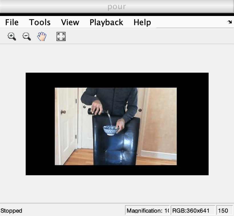
actionLabel = categorical
     pour
score = single
    0.4482
Load Training Data
This example trains an I3D Video Classifier using the HMDB51 data set. Use the downloadHMDB51 supporting function, listed at the end of this example, to download the HMDB51 data set to a folder named hmdb51.
downloadFolder = fullfile(tempdir,"hmdb51");
downloadHMDB51(downloadFolder);
After the download is complete, extract the RAR file hmdb51_org.rar to the hmdb51 folder. Next, use the checkForHMDB51Folder supporting function, listed at the end of this example, to confirm that the downloaded and extracted files are in place.
allClasses = checkForHMDB51Folder(downloadFolder);
The data set contains about 2 GB of video data for 7000 clips over 51 classes, such as drink, run, and shake hands. Each video frame has a height of 240 pixels and a minimum width of 176 pixels. The number of frames ranges from 18 to approximately 1000.
To reduce training time, this example trains an activity recognition network to classify 5 action classes instead of all 51 classes in the data set. Set useAllData to true to train with all 51 classes.
useAllData = false;

if useAllData
    classes = allClasses;
end
dataFolder = fullfile(downloadFolder, "hmdb51_org");
Split the data set into a training set for training the classifier, and a test set for evaluating the classifier. Use 80% of the data for the training set and the rest for the test set. Use folders2labels and splitlabels to create label information from folders and split the data based on each label into training and test data sets by randomly selecting a proportion of files from each label.
[labels,files] = folders2labels(fullfile(dataFolder,string(classes)),...
    "IncludeSubfolders",true,...
    "FileExtensions",'.avi');

indices = splitlabels(labels,0.8,'randomized');

trainFilenames = files(indices{1});
testFilenames  = files(indices{2});
To normalize the input data for the network, the minimum and maximum values for the data set are provided in the MAT file inputStatistics.mat, attached to this example. To find the minimum and maximum values for a different data set, use the inputStatistics supporting function, listed at the end of this example.
inputStatsFilename = 'inputStatistics.mat';
if ~exist(inputStatsFilename, 'file')
    disp("Reading all the training data for input statistics...")
    inputStats = inputStatistics(dataFolder);
else
    d = load(inputStatsFilename);
    inputStats = d.inputStats;
end
Load Dataset
This example uses a datastore to read the videos scenes, the corresponding optical flow data, and the corresponding labels from the video files.
Specify the number of video frames the datastore should be configured to output for each time data is read from the datastore.
numFrames = 64;
A value of 64 is used here to balance memory usage and classification time. Common values to consider are 16, 32, 64, or 128. Using more frames helps capture additional temporal information, but requires more memory. You might need to lower this value depending on your system resources. Empirical analysis is required to determine the optimal number of frames.
Next, specify the height and width of the frames the datastore should be configured to output. The datastore automatically resizes the raw video frames to the specified size to enable batch processing of multiple video sequences.
frameSize = [112,112];
A value of [112 112] is used to capture longer temporal relationships in the video scene which help classify activities with long time durations. Common values for the size are [112 112], [224 224], or [256 256]. Smaller sizes enable the use of more video frames at the cost of memory usage, processing time, and spatial resolution. The minimum height and width of the video frames in the HMDB51 data set are 240 and 176, respectively. If you want to specify a frame size for the datastore to read that is larger than the minimum values, such as [256, 256], first resize the frames using imresize. As with the number of frames, empirical analysis is required to determine the optimal values.
Specify the number of channels as 3 for the RGB video subnetwork, and 2 for the optical flow subnetwork of the I3D video classifier. The two channels for optical flow data are the and components of velocity, and , respectively.
rgbChannels = 3;
flowChannels = 2;
Use the helper function, createFileDatastore, to configure two FileDatastore objects for loading the data, one for training and another for validation. The helper function is listed at the end of this example. Each datastore reads a video file to provide RGB data and the corresponding label information.
isDataForTraining = true;
dsTrain = createFileDatastore(trainFilenames,numFrames,rgbChannels,classes,isDataForTraining);

isDataForTraining = false;
dsVal = createFileDatastore(testFilenames,numFrames,rgbChannels,classes,isDataForTraining);
Configure I3D Video Classifier
Define Network Architecture
I3D network
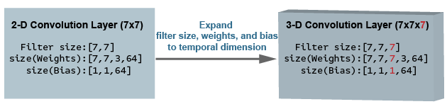
Using a 3-D CNN is a natural approach to extracting spatio-temporal features from videos. You can create an I3D network from a pretrained 2-D image classification network such as Inception v1 or ResNet-50 by expanding 2-D filters and pooling kernels into 3-D. This procedure reuses the weights learned from the image classification task to bootstrap the video recognition task.
The following figure is a sample showing how to inflate a 2-D convolution layer to a 3-D convolution layer. The inflation involves expanding the filter size, weights, and bias by adding a third dimension (the temporal dimension).
Two-Stream I3D Network
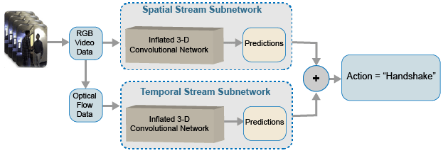
Video data can be considered to have two parts: a spatial component and a temporal component.
The spatial component comprises information about the shape, texture, and color of objects in video. RGB data contains this information.
The temporal component comprises information about the motion of objects across the frames and depicts important movements between the camera and the objects in a scene. Computing optical flow is a common technique for extracting temporal information from video.
A two-stream CNN incorporates a spatial subnetwork and a temporal subnetwork [2]. A convolutional neural network trained on dense optical flow and a video data stream can achieve better performance with limited training data than with raw stacked RGB frames. The following illustration shows a typical two-stream I3D network.
In this example, you create an I3D video classifier based on the GoogLeNet architecture, a 3D Convolution Neural Network Video Classifier pretrained on the Kinetics-400 dataset.
Specify GoogLeNet as the backbone convolution neural network architecture for the I3D video classifier that contains two subnetworks, one for video data and another for optical flow data.
baseNetwork = "googlenet-video-flow";Specify the input size for the Inflated-3D Video Classifier.
inputSize = [frameSize, rgbChannels, numFrames];
Obtain the minimum and maximum values for the RGB and optical flow data from the inputStats structure loaded from the inputStatistics.mat file. These values are needed to normalize the input data.
oflowMin = squeeze(inputStats.oflowMin)';
oflowMax = squeeze(inputStats.oflowMax)';
rgbMin   = squeeze(inputStats.rgbMin)';
rgbMax   = squeeze(inputStats.rgbMax)';

stats.Video.Min               = rgbMin;
stats.Video.Max               = rgbMax;
stats.Video.Mean              = [];
stats.Video.StandardDeviation = [];

stats.OpticalFlow.Min               = oflowMin(1:flowChannels);
stats.OpticalFlow.Max               = oflowMax(1:flowChannels);
stats.OpticalFlow.Mean              = [];
stats.OpticalFlow.StandardDeviation = [];
Create the I3D Video Classifier by using the inflated3dVideoClassifier function.
i3d = inflated3dVideoClassifier(baseNetwork,string(classes),...
    "InputSize",inputSize,...
    "InputNormalizationStatistics",stats);
Specify a model name for the video classifier.
i3d.ModelName = "Inflated-3D Activity Recognizer Using Video and Optical Flow";Prepare Data for Training
Data augmentation provides a way to use limited data sets for training. Augmentation on video data must be the same for a collection of frames, i.e. a video sequence, based on the network input size. Minor changes, such as translation, cropping, or transforming an image, provide, new, distinct, and unique images that you can use to train a robust video classifier. Datastores are a convenient way to read and augment collections of data. Augment the training video data by using the augmentVideo supporting function, defined at the end of this example.
dsTrain = transform(dsTrain, @augmentVideo);
Preprocess the training video data to resize to the I3D Video Classifier input size, by using the preprocessVideoClips, defined at the end of this example. Specify the InputNormalizationStatistics property of the video classifier and input size to the preprocessing function as field values in a struct, preprocessInfo. The InputNormalizationStatistics property is used to rescale the video frames and optical flow data between -1 and 1. The input size is used to resize the video frames using imresize based on the SizingOption value in the info struct. Alternatively, you could use "randomcrop" or "centercrop" to random crop or center crop the input data to the input size of the video classifier. Note that data augmentation is not applied to the test and validation data. Ideally, test and validation data should be representative of the original data and is left unmodified for unbiased evaluation.
preprocessInfo.Statistics = i3d.InputNormalizationStatistics;
preprocessInfo.InputSize = inputSize;
preprocessInfo.SizingOption = "resize";
dsTrain = transform(dsTrain, @(data)preprocessVideoClips(data, preprocessInfo));
dsVal = transform(dsVal, @(data)preprocessVideoClips(data, preprocessInfo));
Train I3D Video Classifier
This section of the example shows how the video classifier shown above is trained using transfer learning. Set the doTraining variable to false to use the pretrained video classifier without having to wait for training to complete. Alternatively, if you want to train the video classifier, set the doTraining variable to true.
doTraining = false;
Define Model Gradients Function
Create the supporting function modelGradients, listed at the end of this example. The modelGradients function takes as input the I3D video classifier i3d, a mini-batch of input data dlRGB and dlFlow, and a mini-batch of ground truth label data dlY. The function returns the training loss value, the gradients of the loss with respect to the learnable parameters of the classifier, and the mini-batch accuracy of the classifier.
The loss is calculated by computing the average of the cross-entropy losses of the predictions from each of the subnetworks. The output predictions of the network are probabilities between 0 and 1 for each of the classes.
The accuracy of each of the classifier is calculated by taking the average of the RGB and optical flow predictions, and comparing it to the ground truth label of the inputs.
Specify Training Options
Train with a mini-batch size of 20 for 600 iterations. Specify the iteration after which to save the video classifier with the best validation accuracy by using the SaveBestAfterIteration parameter.
Specify the cosine-annealing learning rate schedule [3] parameters:
A minimum learning rate of 1e-4.
A maximum learning rate of 1e-3.
Cosine number of iterations of 100, 200, and 300, after which the learning rate schedule cycle restarts. The option
CosineNumIterationsdefines the width of each cosine cycle.
Specify the parameters for SGDM optimization. Initialize the SGDM optimization parameters at the beginning of the training:
A momentum of 0.9.
An initial velocity parameter initialized as
[].An L2 regularization factor of 0.0005.
Specify to dispatch the data in the background using a parallel pool. If DispatchInBackground is set to true, open a parallel pool with the specified number of parallel workers, and create a DispatchInBackgroundDatastore, provided as part of this example, that dispatches the data in the background to speed up training using asynchronous data loading and preprocessing. By default, this example uses a GPU if one is available. Otherwise, it uses a CPU. Using a GPU requires Parallel Computing Toolbox™ and a CUDA® enabled NVIDIA® GPU. For information about the supported compute capabilities, see GPU Computing Requirements (Parallel Computing Toolbox).
params.Classes = classes;
params.MiniBatchSize = 20;
params.NumIterations = 600;
params.SaveBestAfterIteration = 400;
params.CosineNumIterations = [100, 200, 300];
params.MinLearningRate = 1e-4;
params.MaxLearningRate = 1e-3;
params.Momentum = 0.9;
params.VelocityRGB = [];
params.VelocityFlow = [];
params.L2Regularization = 0.0005;
params.ProgressPlot = true;
params.Verbose = true;
params.ValidationData = dsVal;
params.DispatchInBackground = false;
params.NumWorkers = 4;
Train the I3D video classifier using the RGB video data and optical flow data.
For each epoch:
Shuffle the data before looping over mini-batches of data.
Use
minibatchqueueto loop over the mini-batches. The supporting functioncreateMiniBatchQueue, listed at the end of this example, uses the given training datastore to create aminibatchqueue.Use the validation data
dsValto validate the networks.Display the loss and accuracy results for each epoch using the supporting function
displayVerboseOutputEveryEpoch, listed at the end of this example.
For each mini-batch:
Convert the video data or optical flow data and the labels to
dlarrayobjects with the underlying type single.To enable processing the time dimension of the video data using the I3D Video Classifier specify the temporal sequence dimension,
"T". Specify the dimension labels"SSCTB"(spatial, spatial, channel, temporal, batch) for the video data, and"CB"for the label data.
The minibatchqueue object uses the supporting function batchVideoAndFlow, listed at the end of this example, to batch the RGB video and optical flow data.
params.ModelFilename = "inflated3d-FiveClasses-hmdb51.mat";
if doTraining
    epoch     = 1;
    bestLoss  = realmax;

    accTrain     = [];
    accTrainRGB  = [];
    accTrainFlow = [];
    lossTrain    = [];

    iteration = 1;
    start     = tic;
    trainTime = start;
    shuffled  = shuffleTrainDs(dsTrain);

    % Number of outputs is three: One for RGB frames, one for optical flow
    % data, and one for ground truth labels.
    numOutputs = 3;
    mbq        = createMiniBatchQueue(shuffled, numOutputs, params);

    % Use the initializeTrainingProgressPlot and initializeVerboseOutput
    % supporting functions, listed at the end of the example, to initialize
    % the training progress plot and verbose output to display the training
    % loss, training accuracy, and validation accuracy.
    plotters = initializeTrainingProgressPlot(params);
    initializeVerboseOutput(params);

    while iteration <= params.NumIterations

        % Iterate through the data set.
        [dlVideo,dlFlow,dlY] = next(mbq);

        % Evaluate the model gradients and loss using dlfeval.
        [gradRGB,gradFlow,loss,acc,accRGB,accFlow,stateRGB,stateFlow] = ...
            dlfeval(@modelGradients,i3d,dlVideo,dlFlow,dlY);

        % Accumulate the loss and accuracies.
        lossTrain    = [lossTrain, loss];
        accTrain     = [accTrain, acc];
        accTrainRGB  = [accTrainRGB, accRGB];
        accTrainFlow = [accTrainFlow, accFlow];

        % Update the network state.
        i3d.VideoState       = stateRGB;
        i3d.OpticalFlowState = stateFlow;

        % Update the gradients and parameters for the RGB and optical flow
        % subnetworks using the SGDM optimizer.
        [i3d.VideoLearnables,params.VelocityRGB] = ...
            updateLearnables(i3d.VideoLearnables,gradRGB,params,params.VelocityRGB,iteration);
        [i3d.OpticalFlowLearnables,params.VelocityFlow,learnRate] = ...
            updateLearnables(i3d.OpticalFlowLearnables,gradFlow,params,params.VelocityFlow,iteration);

        if ~hasdata(mbq) || iteration == params.NumIterations
            % Current epoch is complete. Do validation and update progress.
            trainTime = toc(trainTime);

            [validationTime,cmat,lossValidation,accValidation,accValidationRGB,accValidationFlow] = ...
                doValidation(params, i3d);

            accTrain     = mean(accTrain);
            accTrainRGB  = mean(accTrainRGB);
            accTrainFlow = mean(accTrainFlow);
            lossTrain    = mean(lossTrain);

            % Update the training progress.
            displayVerboseOutputEveryEpoch(params,start,learnRate,epoch,iteration,...
                accTrain,accTrainRGB,accTrainFlow,...
                accValidation,accValidationRGB,accValidationFlow,...
                lossTrain,lossValidation,trainTime,validationTime);
            updateProgressPlot(params,plotters,epoch,iteration,start,lossTrain,accTrain,accValidation);

            % Save the trained video classifier and the parameters, that gave
            % the best validation loss so far. Use the saveData supporting function,
            % listed at the end of this example.
            bestLoss = saveData(i3d,bestLoss,iteration,cmat,lossTrain,lossValidation,...
                accTrain,accValidation,params);
        end

        if ~hasdata(mbq) && iteration < params.NumIterations
            % Current epoch is complete. Initialize the training loss, accuracy
            % values, and minibatchqueue for the next epoch.
            accTrain     = [];
            accTrainRGB  = [];
            accTrainFlow = [];
            lossTrain    = [];

            trainTime  = tic;
            epoch      = epoch + 1;
            shuffled   = shuffleTrainDs(dsTrain);
            numOutputs = 3;
            mbq        = createMiniBatchQueue(shuffled, numOutputs, params);

        end

        iteration = iteration + 1;
    end

    % Display a message when training is complete.
    endVerboseOutput(params);

    disp("Model saved to: " + params.ModelFilename);
end
Evaluate I3D Video Classifier
Use the test data set to evaluate the accuracy of the trained video classifier.
Load the best model saved during training or use the pretrained model.
if doTraining
    transferLearned = load(params.ModelFilename);
    inflated3dPretrained = transferLearned.data.inflated3d;
end
Create a minibatchqueue object to load batches of the test data.
numOutputs = 3;
mbq = createMiniBatchQueue(params.ValidationData, numOutputs, params);
For each batch of test data, make predictions using the RGB and optical flow networks, take the average of the predictions, and compute the prediction accuracy using a confusion matrix.
numClasses = numel(classes);
cmat = sparse(numClasses,numClasses);
while hasdata(mbq)
    [dlRGB, dlFlow, dlY] = next(mbq);

    % Pass the video input as RGB and optical flow data through the
    % two-stream I3D Video Classifier to get the separate predictions.
    [dlYPredRGB,dlYPredFlow] = predict(inflated3dPretrained,dlRGB,dlFlow);

    % Fuse the predictions by calculating the average of the predictions.
    dlYPred = (dlYPredRGB + dlYPredFlow)/2;

    % Calculate the accuracy of the predictions.
    [~,YTest] = max(dlY,[],1);
    [~,YPred] = max(dlYPred,[],1);

    cmat = aggregateConfusionMetric(cmat,YTest,YPred);
end
Compute the average classification accuracy for the trained networks.
accuracyEval = sum(diag(cmat))./sum(cmat,"all")accuracyEval = 0.8850
Display the confusion matrix.
figure
chart = confusionchart(cmat,classes);
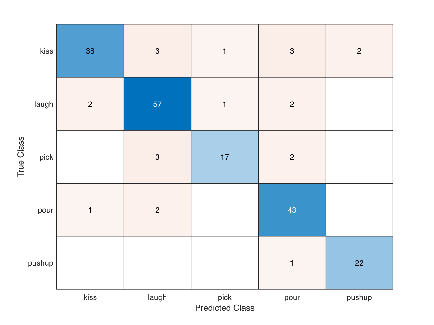
The I3D video classifier that is pretrained on the Kinetics-400 dataset, provides better performance for human activity recognition on transfer learning. The above training was run on 24GB Titan-X GPU for about 100 minutes. When training from scratch on a small activity recognition video dataset, the training time and convergence takes much longer than the pretrained video classifier. Transer learning using the Kinetics-400 pretrained I3D video classifier also avoids overfitting the classifier when ran for larger number of epochs. However, the SlowFast Video Classifier and R(2+1)D Video Classifier that are pretrained on the Kinetics-400 dataset provide better performance and faster convergence during training compared to the I3D Video Classifier. To learn more about video recognition using deep learning, see Getting Started with Video Classification Using Deep Learning (Computer Vision Toolbox).
Supporting Functions
inputStatistics
The inputStatistics function takes as input the name of the folder containing the HMDB51 data, and calculates the minimum and maximum values for the RGB data and the optical flow data. The minimum and maximum values are used as normalization inputs to the input layer of the networks. This function also obtains the number of frames in each of the video files to use later during training and testing the network. In order to find the minimum and maximum values for a different data set, use this function with a folder name containing the data set.
function inputStats = inputStatistics(dataFolder)
    ds = createDatastore(dataFolder);
    ds.ReadFcn = @getMinMax;

    tic;
    tt = tall(ds);
    varnames = {'rgbMax','rgbMin','oflowMax','oflowMin'};
    stats = gather(groupsummary(tt,[],{'max','min'}, varnames));
    inputStats.Filename = gather(tt.Filename);
    inputStats.NumFrames = gather(tt.NumFrames);
    inputStats.rgbMax = stats.max_rgbMax;
    inputStats.rgbMin = stats.min_rgbMin;
    inputStats.oflowMax = stats.max_oflowMax;
    inputStats.oflowMin = stats.min_oflowMin;
    save('inputStatistics.mat','inputStats');
    toc;
end

function data = getMinMax(filename)
    reader = VideoReader(filename);
    opticFlow = opticalFlowFarneback;
    data = [];
    while hasFrame(reader)
        frame = readFrame(reader);
        [rgb,oflow] = findMinMax(frame,opticFlow);
        data = assignMinMax(data, rgb, oflow);
    end

    totalFrames = floor(reader.Duration * reader.FrameRate);
    totalFrames = min(totalFrames, reader.NumFrames);

    [labelName, filename] = getLabelFilename(filename);
    data.Filename = fullfile(labelName, filename);
    data.NumFrames = totalFrames;

    data = struct2table(data,'AsArray',true);
end

function [labelName, filename] = getLabelFilename(filename)
    fileNameSplit = split(filename,'/');
    labelName = fileNameSplit{end-1};
    filename = fileNameSplit{end};
end

function data = assignMinMax(data, rgb, oflow)
    if isempty(data)
        data.rgbMax = rgb.Max;
        data.rgbMin = rgb.Min;
        data.oflowMax = oflow.Max;
        data.oflowMin = oflow.Min;
        return;
    end
    data.rgbMax = max(data.rgbMax, rgb.Max);
    data.rgbMin = min(data.rgbMin, rgb.Min);

    data.oflowMax = max(data.oflowMax, oflow.Max);
    data.oflowMin = min(data.oflowMin, oflow.Min);
end

function [rgbMinMax,oflowMinMax] = findMinMax(rgb, opticFlow)
    rgbMinMax.Max = max(rgb,[],[1,2]);
    rgbMinMax.Min = min(rgb,[],[1,2]);

    gray = rgb2gray(rgb);
    flow = estimateFlow(opticFlow,gray);
    oflow = cat(3,flow.Vx,flow.Vy,flow.Magnitude);

    oflowMinMax.Max = max(oflow,[],[1,2]);
    oflowMinMax.Min = min(oflow,[],[1,2]);
end

function ds = createDatastore(folder)
    ds = fileDatastore(folder,...
        'IncludeSubfolders', true,...
        'FileExtensions', '.avi',...
        'UniformRead', true,...
        'ReadFcn', @getMinMax);
    disp("NumFiles: " + numel(ds.Files));
end
createFileDatastore
The createFileDatastore function creates a FileDatastore object using the given file names. The FileDatastore object reads the data in 'partialfile' mode, so every read can return partially read frames from videos. This feature helps with reading large video files, if all of the frames do not fit in memory.
function datastore = createFileDatastore(trainingFolder,numFrames,numChannels,classes,isDataForTraining)
    readFcn = @(f,u)readVideo(f,u,numFrames,numChannels,classes,isDataForTraining);
    datastore = fileDatastore(trainingFolder,...
        'IncludeSubfolders',true,...
        'FileExtensions','.avi',...
        'ReadFcn',readFcn,...
        'ReadMode','partialfile');
end
shuffleTrainDs
The shuffleTrainDs function shuffles the files present in the training datastore dsTrain.
function shuffled = shuffleTrainDs(dsTrain)
shuffled = copy(dsTrain);
transformed = isa(shuffled, 'matlab.io.datastore.TransformedDatastore');
if transformed
    files = shuffled.UnderlyingDatastores{1}.Files;
else
    files = shuffled.Files;
end
n = numel(files);
shuffledIndices = randperm(n);
if transformed
    shuffled.UnderlyingDatastores{1}.Files = files(shuffledIndices);
else
    shuffled.Files = files(shuffledIndices);
end

reset(shuffled);
end
readVideo
The readVideo function reads video frames, and the corresponding label values for a given video file. During training, the read function reads the specific number of frames as per the network input size, with a randomly chosen starting frame. During testing, all the frames are sequentially read. The video frames are resized to the required classifier network input size for training, and for testing and validation.
function [data,userdata,done] = readVideo(filename,userdata,numFrames,numChannels,classes,isDataForTraining)
    if isempty(userdata)
        userdata.reader      = VideoReader(filename);
        userdata.batchesRead = 0;

        userdata.label = getLabel(filename,classes);

        totalFrames = floor(userdata.reader.Duration * userdata.reader.FrameRate);
        totalFrames = min(totalFrames, userdata.reader.NumFrames);
        userdata.totalFrames = totalFrames;
        userdata.datatype = class(read(userdata.reader,1));
    end
    reader      = userdata.reader;
    totalFrames = userdata.totalFrames;
    label       = userdata.label;
    batchesRead = userdata.batchesRead;

    if isDataForTraining
        video = readForTraining(reader, numFrames, totalFrames);
    else
        video = readForValidation(reader, userdata.datatype, numChannels, numFrames, totalFrames);
    end

    data = {video, label};

    batchesRead = batchesRead + 1;

    userdata.batchesRead = batchesRead;

    if numFrames > totalFrames
        numBatches = 1;
    else
        numBatches = floor(totalFrames/numFrames);
    end
    % Set the done flag to true, if the reader has read all the frames or
    % if it is training.
    done = batchesRead == numBatches || isDataForTraining;
end
readForTraining
The readForTraining function reads the video frames for training the video classifier. The function reads the specific number of frames as per the network input size, with a randomly chosen starting frame. If there are not enough frames left over, the video sequence is repeated to pad the required number of frames.
function video = readForTraining(reader, numFrames, totalFrames)
    if numFrames >= totalFrames
        startIdx = 1;
        endIdx = totalFrames;
    else
        startIdx = randperm(totalFrames - numFrames + 1);
        startIdx = startIdx(1);
        endIdx = startIdx + numFrames - 1;
    end
    video = read(reader,[startIdx,endIdx]);
    if numFrames > totalFrames
        % Add more frames to fill in the network input size.
        additional = ceil(numFrames/totalFrames);
        video = repmat(video,1,1,1,additional);
        video = video(:,:,:,1:numFrames);
    end
end
readForValidation
The readForValidation function reads the video frames for evaluating the trained video classifier. The function reads the specific number of frames sequentially as per the network input size. If there are not enough frames left over, the video sequence is repeated to pad the required number of frames.
function video = readForValidation(reader, datatype, numChannels, numFrames, totalFrames)
    H = reader.Height;
    W = reader.Width;
    toRead = min([numFrames,totalFrames]);
    video = zeros([H,W,numChannels,toRead], datatype);
    frameIndex = 0;
    while hasFrame(reader) && frameIndex < numFrames
        frame = readFrame(reader);
        frameIndex = frameIndex + 1;
        video(:,:,:,frameIndex) = frame;
    end

    if frameIndex < numFrames
        video = video(:,:,:,1:frameIndex);
        additional = ceil(numFrames/frameIndex);
        video = repmat(video,1,1,1,additional);
        video = video(:,:,:,1:numFrames);
    end
end
getLabel
The getLabel function obtains the label name from the full path of a filename. The label for a file is the folder in which it exists. For example, for a file path such as "/path/to/dataset/clapping/video_0001.avi", the label name is "clapping".
function label = getLabel(filename,classes)
    folder = fileparts(string(filename));
    [~,label] = fileparts(folder);
    label = categorical(string(label), string(classes));
end
augmentVideo
The augmentVideo function uses the augment transform function provided by the augmentTransform supporting function to apply the same augmentation across a video sequence.
function data = augmentVideo(data)
    numSequences = size(data,1);
    for ii = 1:numSequences
        video = data{ii,1};
        % HxWxC
        sz = size(video,[1,2,3]);
        % One augmentation per sequence
        augmentFcn = augmentTransform(sz);
        data{ii,1} = augmentFcn(video);
    end
end
augmentTransform
The augmentTransform function creates an augmentation method with random left-right flipping and scaling factors.
function augmentFcn = augmentTransform(sz)
% Randomly flip and scale the image.
tform = randomAffine2d('XReflection',true,'Scale',[1 1.1]);
rout = affineOutputView(sz,tform,'BoundsStyle','CenterOutput');

augmentFcn = @(data)augmentData(data,tform,rout);

    function data = augmentData(data,tform,rout)
        data = imwarp(data,tform,'OutputView',rout);
    end
end
preprocessVideoClips
The preprocessVideoClips function preprocesses the training video data to resize to the I3D Video Classifier input size. It takes the InputNormalizationStatistics and the InputSize properties of the video classifier in a struct, info. The InputNormalizationStatistics property is used to rescale the video frames and optical flow data between -1 and 1. The input size is used to resize the video frames using imresize based on the SizingOption value in the info struct. Alternatively, you could use "randomcrop" or "centercrop" as values for SizingOption to random crop or center crop the input data to the input size of the video classifier.
function preprocessed = preprocessVideoClips(data, info)
inputSize = info.InputSize(1:2);
sizingOption = info.SizingOption;
switch sizingOption
    case "resize"
        sizingFcn = @(x)imresize(x,inputSize);
    case "randomcrop"
        sizingFcn = @(x)cropVideo(x,@randomCropWindow2d,inputSize);
    case "centercrop"
        sizingFcn = @(x)cropVideo(x,@centerCropWindow2d,inputSize);
end
numClips = size(data,1);

rgbMin   = info.Statistics.Video.Min;
rgbMax   = info.Statistics.Video.Max;
oflowMin = info.Statistics.OpticalFlow.Min;
oflowMax = info.Statistics.OpticalFlow.Max;

numChannels = length(rgbMin);
rgbMin   = reshape(rgbMin, 1, 1, numChannels);
rgbMax   = reshape(rgbMax, 1, 1, numChannels);

numChannels = length(oflowMin);
oflowMin = reshape(oflowMin, 1, 1, numChannels);
oflowMax = reshape(oflowMax, 1, 1, numChannels);

preprocessed = cell(numClips, 3);
for ii = 1:numClips
    video   = data{ii,1};
    resized = sizingFcn(video);
    oflow   = computeFlow(resized,inputSize);

    % Cast the input to single.
    resized = single(resized);
    oflow   = single(oflow);

    % Rescale the input between -1 and 1.
    resized = rescale(resized,-1,1,"InputMin",rgbMin,"InputMax",rgbMax);
    oflow   = rescale(oflow,-1,1,"InputMin",oflowMin,"InputMax",oflowMax);

    preprocessed{ii,1} = resized;
    preprocessed{ii,2} = oflow;
    preprocessed{ii,3} = data{ii,2};
end
end

function outData = cropVideo(data, cropFcn, inputSize)
imsz = size(data,[1,2]);
cropWindow = cropFcn(imsz, inputSize);
numFrames = size(data,4);
sz = [inputSize, size(data,3), numFrames];
outData = zeros(sz, 'like', data);
for f = 1:numFrames
    outData(:,:,:,f) = imcrop(data(:,:,:,f), cropWindow);
end
end
computeFlow
The computeFlow function takes as input a video sequence, videoFrames, and computes the corresponding optical flow data opticalFlowData using opticalFlowFarneback. The optical flow data contains two channels, which correspond to the - and - components of velocity.
function opticalFlowData = computeFlow(videoFrames, inputSize)
opticalFlow = opticalFlowFarneback;
numFrames = size(videoFrames,4);
sz = [inputSize, 2, numFrames];
opticalFlowData = zeros(sz, 'like', videoFrames);
for f = 1:numFrames
    gray = rgb2gray(videoFrames(:,:,:,f));
    flow = estimateFlow(opticalFlow,gray);

    opticalFlowData(:,:,:,f) = cat(3,flow.Vx,flow.Vy);
end
end
createMiniBatchQueue
The createMiniBatchQueue function creates a minibatchqueue object that provides miniBatchSize amount of data from the given datastore. It also creates a DispatchInBackgroundDatastore if a parallel pool is open.
function mbq = createMiniBatchQueue(datastore, numOutputs, params)
if params.DispatchInBackground && isempty(gcp('nocreate'))
    % Start a parallel pool, if DispatchInBackground is true, to dispatch
    % data in the background using the parallel pool.
    c = parcluster('local');
    c.NumWorkers = params.NumWorkers;
    parpool('local',params.NumWorkers);
end
p = gcp('nocreate');
if ~isempty(p)
    datastore = DispatchInBackgroundDatastore(datastore, p.NumWorkers);
end
inputFormat(1:numOutputs-1) = "SSCTB";
outputFormat = "CB";
mbq = minibatchqueue(datastore, numOutputs, ...
    "MiniBatchSize", params.MiniBatchSize, ...
    "MiniBatchFcn", @batchVideoAndFlow, ...
    "MiniBatchFormat", [inputFormat,outputFormat]);
end
batchVideoAndFlow
The batchVideoAndFlow function batches the video, optical flow, and label data from cell arrays. It uses onehotencode function to encode ground truth categorical labels into one-hot arrays. The one-hot encoded array contains a 1 in the position corresponding to the class of the label, and 0 in every other position.
function [video,flow,labels] = batchVideoAndFlow(video, flow, labels)
% Batch dimension: 5
video = cat(5,video{:});
flow = cat(5,flow{:});

% Batch dimension: 2
labels = cat(2,labels{:});

% Feature dimension: 1
labels = onehotencode(labels,1);
end
modelGradients
The modelGradients function takes as input a mini-batch of RGB data dlRGB, the corresponding optical flow data dlFlow, and the corresponding target dlY, and returns the corresponding loss, the gradients of the loss with respect to the learnable parameters, and the training accuracy. To compute the gradients, evaluate the modelGradients function using the dlfeval function in the training loop.
function [gradientsRGB,gradientsFlow,loss,acc,accRGB,accFlow,stateRGB,stateFlow] = modelGradients(i3d,dlRGB,dlFlow,Y)

% Pass video input as RGB and optical flow data through the two-stream
% network.
[dlYPredRGB,dlYPredFlow,stateRGB,stateFlow] = forward(i3d,dlRGB,dlFlow);

% Calculate fused loss, gradients, and accuracy for the two-stream
% predictions.
rgbLoss = crossentropy(dlYPredRGB,Y);
flowLoss = crossentropy(dlYPredFlow,Y);
% Fuse the losses.
loss = mean([rgbLoss,flowLoss]);

gradientsRGB = dlgradient(rgbLoss,i3d.VideoLearnables);
gradientsFlow = dlgradient(flowLoss,i3d.OpticalFlowLearnables);

% Fuse the predictions by calculating the average of the predictions.
dlYPred = (dlYPredRGB + dlYPredFlow)/2;

% Calculate the accuracy of the predictions.
[~,YTest] = max(Y,[],1);
[~,YPred] = max(dlYPred,[],1);

acc = gather(extractdata(sum(YTest == YPred)./numel(YTest)));

% Calculate the accuracy of the RGB and flow predictions.
[~,YTest] = max(Y,[],1);
[~,YPredRGB] = max(dlYPredRGB,[],1);
[~,YPredFlow] = max(dlYPredFlow,[],1);

accRGB = gather(extractdata(sum(YTest == YPredRGB)./numel(YTest)));
accFlow = gather(extractdata(sum(YTest == YPredFlow)./numel(YTest)));
end
updateLearnables
The updateLearnables function updates the provided learnables with gradients and other parameters using SGDM optimization function sgdmupdate.
function [learnables,velocity,learnRate] = updateLearnables(learnables,gradients,params,velocity,iteration)
    % Determine the learning rate using the cosine-annealing learning rate schedule.
    learnRate = cosineAnnealingLearnRate(iteration, params);

    % Apply L2 regularization to the weights.
    idx = learnables.Parameter == "Weights";
    gradients(idx,:) = dlupdate(@(g,w) g + params.L2Regularization*w, gradients(idx,:), learnables(idx,:));

    % Update the network parameters using the SGDM optimizer.
    [learnables, velocity] = sgdmupdate(learnables, gradients, velocity, learnRate, params.Momentum);
end
cosineAnnealingLearnRate
The cosineAnnealingLearnRate function computes the learning rate based on the current iteration number, minimum learning rate, maximum learning rate, and number of iterations for annealing [3].
function lr = cosineAnnealingLearnRate(iteration, params)
    if iteration == params.NumIterations
        lr = params.MinLearningRate;
        return;
    end
    cosineNumIter = [0, params.CosineNumIterations];
    csum = cumsum(cosineNumIter);
    block = find(csum >= iteration, 1,'first');
    cosineIter = iteration - csum(block - 1);
    annealingIteration = mod(cosineIter, cosineNumIter(block));
    cosineIteration = cosineNumIter(block);
    minR = params.MinLearningRate;
    maxR = params.MaxLearningRate;
    cosMult = 1 + cos(pi * annealingIteration / cosineIteration);
    lr = minR + ((maxR - minR) *  cosMult / 2);
end
aggregateConfusionMetric
The aggregateConfusionMetric function incrementally fills a confusion matrix based on the predicted results YPred and the expected results YTest.
function cmat = aggregateConfusionMetric(cmat,YTest,YPred)
YTest = gather(extractdata(YTest));
YPred = gather(extractdata(YPred));
[m,n] = size(cmat);
cmat = cmat + full(sparse(YTest,YPred,1,m,n));
end
doValidation
The doValidation function validates the video classifier using the validation data.
function [validationTime, cmat, lossValidation, accValidation, accValidationRGB, accValidationFlow] = doValidation(params, i3d)

validationTime = tic;

numOutputs = 3;
mbq = createMiniBatchQueue(params.ValidationData, numOutputs, params);

lossValidation = [];
numClasses = numel(params.Classes);
cmat = sparse(numClasses,numClasses);
cmatRGB = sparse(numClasses,numClasses);
cmatFlow = sparse(numClasses,numClasses);
while hasdata(mbq)

    [dlX1,dlX2,dlY] = next(mbq);

    [loss,YTest,YPred,YPredRGB,YPredFlow] = predictValidation(i3d,dlX1,dlX2,dlY);

    lossValidation = [lossValidation,loss];
    cmat = aggregateConfusionMetric(cmat,YTest,YPred);
    cmatRGB = aggregateConfusionMetric(cmatRGB,YTest,YPredRGB);
    cmatFlow = aggregateConfusionMetric(cmatFlow,YTest,YPredFlow);
end
lossValidation = mean(lossValidation);
accValidation = sum(diag(cmat))./sum(cmat,"all");
accValidationRGB = sum(diag(cmatRGB))./sum(cmatRGB,"all");
accValidationFlow = sum(diag(cmatFlow))./sum(cmatFlow,"all");

validationTime = toc(validationTime);
end
predictValidation
The predictValidation function calculates the loss and prediction values using the provided video classifier for RGB and optical flow data.
function [loss,YTest,YPred,YPredRGB,YPredFlow] = predictValidation(i3d,dlRGB,dlFlow,Y)

% Pass the video input through the two-stream Inflated-3D video classifier.
[dlYPredRGB,dlYPredFlow] = predict(i3d,dlRGB,dlFlow);

% Calculate the cross-entropy separately for the two-stream outputs.
rgbLoss = crossentropy(dlYPredRGB,Y);
flowLoss = crossentropy(dlYPredFlow,Y);

% Fuse the losses.
loss = mean([rgbLoss,flowLoss]);

% Fuse the predictions by calculating the average of the predictions.
dlYPred = (dlYPredRGB + dlYPredFlow)/2;

% Calculate the accuracy of the predictions.
[~,YTest] = max(Y,[],1);
[~,YPred] = max(dlYPred,[],1);

[~,YPredRGB] = max(dlYPredRGB,[],1);
[~,YPredFlow] = max(dlYPredFlow,[],1);

end
saveData
The saveData function saves the given Inflated-3d Video Classifier, accuracy, loss, and other training parameters to a MAT-file.
function bestLoss = saveData(inflated3d,bestLoss,iteration,cmat,lossTrain,lossValidation,...
                accTrain,accValidation,params)
if iteration >= params.SaveBestAfterIteration
    lossValidtion = extractdata(gather(lossValidation));
    if lossValidtion < bestLoss
        params = rmfield(params, 'VelocityRGB');
        params = rmfield(params, 'VelocityFlow');
        bestLoss = lossValidtion;
        inflated3d = gatherFromGPUToSave(inflated3d);
        data.BestLoss = bestLoss;
        data.TrainingLoss = extractdata(gather(lossTrain));
        data.TrainingAccuracy = accTrain;
        data.ValidationAccuracy = accValidation;
        data.ValidationConfmat= cmat;
        data.inflated3d = inflated3d;
        data.Params = params;
        save(params.ModelFilename, 'data');
    end
end
end
gatherFromGPUToSave
The gatherFromGPUToSave function gathers data from the GPU in order to save the video classifier to disk.
function classifier = gatherFromGPUToSave(classifier)
if ~canUseGPU
    return;
end
p = string(properties(classifier));
p = p(endsWith(p, ["Learnables","State"]));
for jj = 1:numel(p)
    prop = p(jj);
    classifier.(prop) = gatherValues(classifier.(prop));
end
    function tbl = gatherValues(tbl)
        for ii = 1:height(tbl)
            tbl.Value{ii} = gather(tbl.Value{ii});
        end
    end
end
checkForHMDB51Folder
The checkForHMDB51Folder function checks for the downloaded data in the download folder.
function classes = checkForHMDB51Folder(dataLoc)
hmdbFolder = fullfile(dataLoc, "hmdb51_org");
if ~isfolder(hmdbFolder)
    error("Download 'hmdb51_org.rar' file using the supporting function 'downloadHMDB51' before running the example and extract the RAR file.");
end

classes = ["brush_hair","cartwheel","catch","chew","clap","climb","climb_stairs",...
    "dive","draw_sword","dribble","drink","eat","fall_floor","fencing",...
    "flic_flac","golf","handstand","hit","hug","jump","kick","kick_ball",...
    "kiss","laugh","pick","pour","pullup","punch","push","pushup","ride_bike",...
    "ride_horse","run","shake_hands","shoot_ball","shoot_bow","shoot_gun",...
    "sit","situp","smile","smoke","somersault","stand","swing_baseball","sword",...
    "sword_exercise","talk","throw","turn","walk","wave"];
expectFolders = fullfile(hmdbFolder, classes);
if ~all(arrayfun(@(x)exist(x,'dir'),expectFolders))
    error("Download hmdb51_org.rar using the supporting function 'downloadHMDB51' before running the example and extract the RAR file.");
end
end
downloadHMDB51
The downloadHMDB51 function downloads the data set and saves it to a directory.
function downloadHMDB51(dataLoc)

if nargin == 0
    dataLoc = pwd;
end
dataLoc = string(dataLoc);

if ~isfolder(dataLoc)
    mkdir(dataLoc);
end

dataUrl     = "http://serre-lab.clps.brown.edu/wp-content/uploads/2013/10/hmdb51_org.rar";
options     = weboptions('Timeout', Inf);
rarFileName = fullfile(dataLoc, 'hmdb51_org.rar');

% Download the RAR file and save it to the download folder.
if ~isfile(rarFileName)
    disp("Downloading hmdb51_org.rar (2 GB) to the folder:")
    disp(dataLoc)
    disp("This download can take a few minutes...")
    websave(rarFileName, dataUrl, options);
    disp("Download complete.")
    disp("Extract the hmdb51_org.rar file contents to the folder: ")
    disp(dataLoc)
end
end
initializeTrainingProgressPlot
The initializeTrainingProgressPlot function configures two plots for displaying the training loss, training accuracy, and validation accuracy.
function plotters = initializeTrainingProgressPlot(params)
if params.ProgressPlot
    % Plot the loss, training accuracy, and validation accuracy.
    figure

    % Loss plot
    subplot(2,1,1)
    plotters.LossPlotter = animatedline;
    xlabel("Iteration")
    ylabel("Loss")

    % Accuracy plot
    subplot(2,1,2)
    plotters.TrainAccPlotter = animatedline('Color','b');
    plotters.ValAccPlotter = animatedline('Color','g');
    legend('Training Accuracy','Validation Accuracy','Location','northwest');
    xlabel("Iteration")
    ylabel("Accuracy")
else
    plotters = [];
end
end
updateProgressPlot
The updateProgressPlot function updates the progress plot with loss and accuracy information during training.
function updateProgressPlot(params,plotters,epoch,iteration,start,lossTrain,accuracyTrain,accuracyValidation)
if params.ProgressPlot

    % Update the training progress.
    D = duration(0,0,toc(start),"Format","hh:mm:ss");
    title(plotters.LossPlotter.Parent,"Epoch: " + epoch + ", Elapsed: " + string(D));
    addpoints(plotters.LossPlotter,iteration,double(gather(extractdata(lossTrain))));
    addpoints(plotters.TrainAccPlotter,iteration,accuracyTrain);
    addpoints(plotters.ValAccPlotter,iteration,accuracyValidation);
    drawnow
end
end
initializeVerboseOutput
The initializeVerboseOutput function displays the column headings for the table of training values, which shows the epoch, mini-batch accuracy, and other training values.
function initializeVerboseOutput(params)
if params.Verbose
    disp(" ")
    if canUseGPU
        disp("Training on GPU.")
    else
        disp("Training on CPU.")
    end
    p = gcp('nocreate');
    if ~isempty(p)
        disp("Training on parallel cluster '" + p.Cluster.Profile + "'. ")
    end
    disp("NumIterations:" + string(params.NumIterations));
    disp("MiniBatchSize:" + string(params.MiniBatchSize));
    disp("Classes:" + join(string(params.Classes), ","));
    disp("|=======================================================================================================================================================================|")
    disp("| Epoch | Iteration | Time Elapsed |     Mini-Batch Accuracy    |    Validation Accuracy     | Mini-Batch | Validation |  Base Learning  | Train Time | Validation Time |")
    disp("|       |           |  (hh:mm:ss)  |       (Avg:RGB:Flow)       |       (Avg:RGB:Flow)       |    Loss    |    Loss    |      Rate       | (hh:mm:ss) |   (hh:mm:ss)    |")
    disp("|=======================================================================================================================================================================|")
end
end
displayVerboseOutputEveryEpoch
The displayVerboseOutputEveryEpoch function displays the verbose output of the training values, such as the epoch, mini-batch accuracy, validation accuracy, and mini-batch loss.
function displayVerboseOutputEveryEpoch(params,start,learnRate,epoch,iteration,...
    accTrain,accTrainRGB,accTrainFlow,accValidation,accValidationRGB,accValidationFlow,lossTrain,lossValidation,trainTime,validationTime)
if params.Verbose
    D = duration(0,0,toc(start),'Format','hh:mm:ss');
    trainTime = duration(0,0,trainTime,'Format','hh:mm:ss');
    validationTime = duration(0,0,validationTime,'Format','hh:mm:ss');

    lossValidation = gather(extractdata(lossValidation));
    lossValidation = compose('%.4f',lossValidation);

    accValidation = composePadAccuracy(accValidation);
    accValidationRGB = composePadAccuracy(accValidationRGB);
    accValidationFlow = composePadAccuracy(accValidationFlow);

    accVal = join([accValidation,accValidationRGB,accValidationFlow], " : ");

    lossTrain = gather(extractdata(lossTrain));
    lossTrain = compose('%.4f',lossTrain);

    accTrain = composePadAccuracy(accTrain);
    accTrainRGB = composePadAccuracy(accTrainRGB);
    accTrainFlow = composePadAccuracy(accTrainFlow);

    accTrain = join([accTrain,accTrainRGB,accTrainFlow], " : ");
    learnRate = compose('%.13f',learnRate);

    disp("| " + ...
        pad(string(epoch),5,'both') + " | " + ...
        pad(string(iteration),9,'both') + " | " + ...
        pad(string(D),12,'both') + " | " + ...
        pad(string(accTrain),26,'both') + " | " + ...
        pad(string(accVal),26,'both') + " | " + ...
        pad(string(lossTrain),10,'both') + " | " + ...
        pad(string(lossValidation),10,'both') + " | " + ...
        pad(string(learnRate),13,'both') + " | " + ...
        pad(string(trainTime),10,'both') + " | " + ...
        pad(string(validationTime),15,'both') + " |")
end

    function acc = composePadAccuracy(acc)
        acc = compose('%.2f',acc*100) + "%";
        acc = pad(string(acc),6,'left');
    end

end
endVerboseOutput
The endVerboseOutput function displays the end of verbose output during training.
function endVerboseOutput(params)
if params.Verbose
    disp("|=======================================================================================================================================================================|")
end
end
References
[1] Carreira, Joao, and Andrew Zisserman. "Quo Vadis, Action Recognition? A New Model and the Kinetics Dataset." Proceedings of the IEEE Conference on Computer Vision and Pattern Recognition (CVPR): 6299??6308. Honolulu, HI: IEEE, 2017.
[2] Simonyan, Karen, and Andrew Zisserman. "Two-Stream Convolutional Networks for Action Recognition in Videos." Advances in Neural Information Processing Systems 27, Long Beach, CA: NIPS, 2017.
[3] Loshchilov, Ilya, and Frank Hutter. "SGDR: Stochastic Gradient Descent with Warm Restarts." International Conferencee on Learning Representations 2017. Toulon, France: ICLR, 2017.
[4] Du Tran, Heng Wang, Lorenzo Torresani, Jamie Ray, Yann LeCun, Manohar Paluri. "A Closer Look at Spatiotemporal Convolutions for Action Recognition". Proceedings of the IEEE Conference on Computer Vision and Pattern Recognition (CVPR), 2018, pp. 6450-6459.
[5] Christoph Feichtenhofer, Haoqi Fan, Jitendra Malik, and Kaiming He. "SlowFast Networks for Video Recognition." Proceedings of the IEEE Conference on Computer Vision and Pattern Recognition (CVPR), 2019.
[6] Will Kay, Joao Carreira, Karen Simonyan, Brian Zhang, Chloe Hillier, Sudheendra Vijayanarasimhan, Fabio Viola, Tim Green, Trevor Back, Paul Natsev, Mustafa Suleyman, Andrew Zisserman. "The Kinetics Human Action Video Dataset." arXiv preprint arXiv:1705.06950, 2017.