Analyze and Compress 1-D Convolutional Neural Network

Since R2024b

This example uses:

This example shows how to analyze and compress a 1-D convolutional neural network used to estimate the frequency of complex-valued waveforms.

The network used in this example is a sequence-to-one regression network using the Complex Waveform data set, which contains 500 synthetically generated complex-valued waveforms of varying lengths with two channels. The network predicts the frequency of the waveforms.

The network in this example takes up about 45 KB of memory. If you want to use this model for inference, but have a memory restriction such as a limited-resource hardware target on which to embed the model, then you can compress the model. You can use the same techniques to compress much larger networks.

The example workflow consists of five steps.

Load a pretrained network.
To understand the potential effects of compression on the network, analyze the network for compression using Deep Network Designer.
Compress the network using Taylor pruning.
Compress the network further using projection.
Compare the size and performance of the different networks.

For more information on how to train the 1-D convolutional neural network used in this example, see Train Network with Complex-Valued Data.

Load and Explore Network and Data

Load the network, training data, validation data, and test data.

load("ComplexValuedSequenceDataAndNetwork.mat")

Compare the frequencies predicted by the pretrained network to the true frequencies for the first few sample sequences from the test set.

TPred = minibatchpredict(net,XTest, ...
    SequencePaddingDirection="left", ...
    InputDataFormats="CTB");

numChannels = 2;
displayLabels = [ ...
    "Real Part" + newline + "Channel " + string(1:numChannels), ...
    "Imaginary Part" + newline + "Channel " + string(1:numChannels)];

figure
tiledlayout(2,2)
for i = 1:4
    nexttile

    stackedplot([real(XTest{i}') imag(XTest{i}')], DisplayLabels=displayLabels);
    
    xlabel("Time Step")
    title(["Predicted Frequency: " + TPred(i);"True Frequency: " + TTest(i)])
end

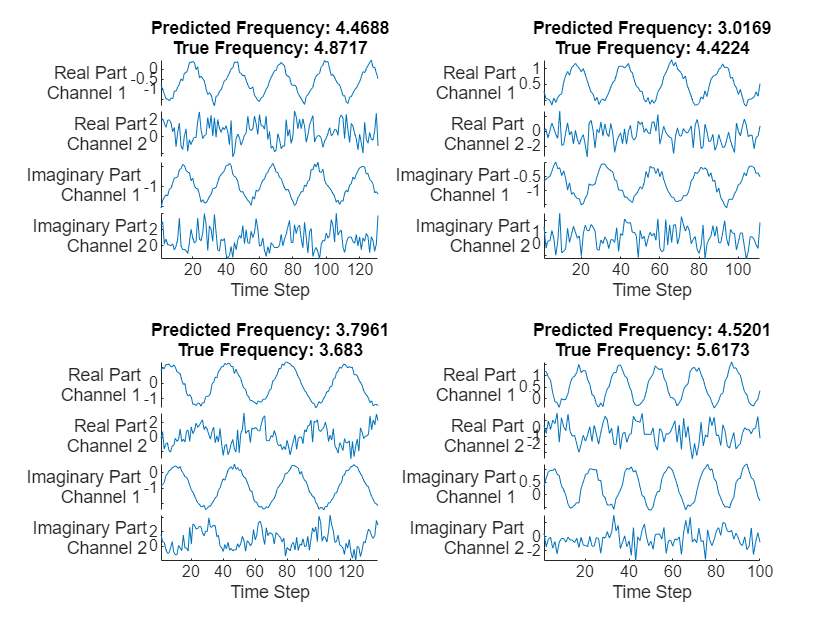
Calculate the root mean squared error of the network on the test data using the testnet function. Later, you use this value to verify that the compressed network is as accurate as the original network.

rmseOriginalNetwork = testnet(net,XTest,TTest,"rmse",InputDataFormats="CTB")

rmseOriginalNetwork = 
0.8072

Analyze Network for Compression

Open the network in Deep Network Designer.

>> deepNetworkDesigner(net)

Get a report on how much compression pruning or projection of the network can achieve by clicking the Analyze for compression button in the toolstrip.

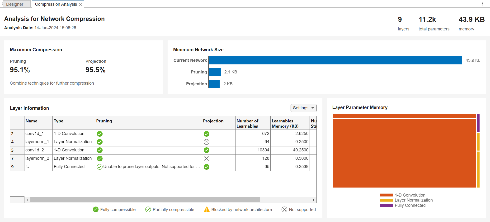
The analysis report shows that you can compress the network using either pruning or projection. You can also use a combination of both techniques. If you use both techniques, the simplest workflow is to first perform pruning and then projection.

Compress Network Using Pruning

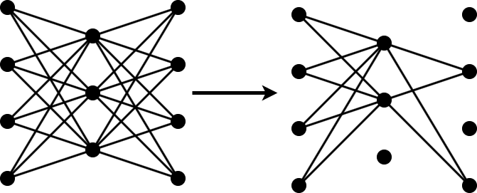
To prune a convolutional network using Taylor pruning in MATLAB, iterate over the following two steps until the network size fulfills your requirements.

Determine the importance scores of the prunable filters and remove the least important filters by applying a pruning mask.
Retrain the network for several iterations with the updated pruning mask.

Then, use the final pruning mask to update the network architecture.

Prepare Data for Pruning

First, create a mini-batch queue that processes and manages mini-batches of training sequences during pruning and retraining.

cds = combine(arrayDatastore(XTrain,OutputType="same"),arrayDatastore(TTrain,OutputType="cell"));
mbqPrune = minibatchqueue(cds,2, ...
    PartialMiniBatch = "discard", ...
    MiniBatchFcn = @preprocessPruningMiniBatch, ...
    MiniBatchFormat = ["CTB","BC"]);

function [X,T] = preprocessPruningMiniBatch(XCell,TCell)
    X = padsequences(XCell,2,Direction="left");
    T = cell2mat(TCell);
end

Create a Taylor prunable network from the pretrained network using the taylorPrunableNetwork function.

netPrunable = taylorPrunableNetwork(net);

View the number of convolution filters in the network that are suitable for pruning.

netPrunable.NumPrunables

ans = 
78

Set the pruning options. Choosing the pruning options requires empirical analysis and depends on your requirements for network size and accuracy.

numPruningIterations specifies the number of iterations to use for the pruning process.
maxToPrune specifies the maximum number of filters to prune in each iteration of the pruning loop. In total, a maximum of numPruningIterations * maxToPrune filters are pruned. Note that the filters do not all contain the same number of learnable parameters.
numRetrainingEpochs specifies the number of epochs to use for retraining during each iteration of the pruning loop.
initialLearnRate specifies the initial learning rate used for retraining during each iteration of the pruning loop.

numPruningIterations = 5;
maxToPrune = 8;
numRetrainingEpochs = 15;
initialLearnRate = 0.01;

Prune Pretrained Network

Each pruning iteration consists of two steps.

First, retrain the network for numRetrainingEpochs epochs to fine-tune it. During the last retraining epoch, compute the importance scores of the prunable filters using the updateScore function. You can do so inside the custom retraining loop because both steps require iterating over either the entire mini-batch queue or a representative subset. Both steps also require that you compute the activations and gradients of the network.

Second, update the pruning mask using the updatePrunables function.

iteration = 0;
for ii = 1:numPruningIterations
    tic;

    % Initialize input arguments for adamupdate
    averageGrad = [];
    averageSqGrad = [];
    fineTuningIteration = 0;    
    
    % Retrain network
    for jj = 1:numRetrainingEpochs
        reset(mbqPrune);
        shuffle(mbqPrune);
        while hasdata(mbqPrune)
            fineTuningIteration = fineTuningIteration+1;

            [X, T] = next(mbqPrune);

            [~,state,gradients,pruningActivations,pruningGradients] = dlfeval(@modelLoss,netPrunable,X,T);
            netPrunable.State = state;

            [netPrunable,averageGrad,averageSqGrad] = adamupdate(netPrunable, gradients,...
                averageGrad,averageSqGrad, fineTuningIteration, initialLearnRate);

            % In last retraining epoch, compute importance scores
            if jj==numRetrainingEpochs
                netPrunable = updateScore(netPrunable,pruningActivations,pruningGradients);
            end
        end
    end

        % Update pruning mask
        netPrunable = updatePrunables(netPrunable,MaxToPrune=maxToPrune);

    t = toc;
    disp("Iteration "+ii+"/"+numPruningIterations+" complete. Elapsed time is "+t+" seconds.")
end

Iteration 1/5 complete. Elapsed time is 10.813 seconds.
Iteration 2/5 complete. Elapsed time is 2.9865 seconds.
Iteration 3/5 complete. Elapsed time is 2.6516 seconds.
Iteration 4/5 complete. Elapsed time is 3.0495 seconds.
Iteration 5/5 complete. Elapsed time is 2.5111 seconds.

Analyze the pruned network using the analyzeNetwork function. View information about the pruned layers.

info = analyzeNetwork(netPrunable,Plots="none");
info.LayerInfo(info.LayerInfo.LearnablesReduction>0,["Name" "Type" "NumLearnables" "LearnablesReduction" "NumPrunedFilters"])

ans=5×5 table
        Name                 Type             NumLearnables    LearnablesReduction    NumPrunedFilters
    _____________    _____________________    _____________    ___________________    ________________

    "conv1d_1"       "1-D Convolution"             378                0.4375                 14       
    "layernorm_1"    "Layer Normalization"          36                0.4375                  0       
    "conv1d_2"       "1-D Convolution"            3458                0.6644                 26       
    "layernorm_2"    "Layer Normalization"          76               0.40625                  0       
    "fc"             "Fully Connected"              39                   0.4                  0

Convert the network back into a dlnetwork object.

netPruned = dlnetwork(netPrunable);

Retrain Pruned Network

Test the pruned network. Compare the RMSE of the pruned and original networks.

rmsePrunedNetwork = testnet(netPruned,XTest,TTest,"rmse",InputDataFormats="CTB")

rmsePrunedNetwork = 
4.0924

rmseOriginalNetwork

rmseOriginalNetwork = 
0.8072

Retrain the pruned network to regain some of the lost accuracy.

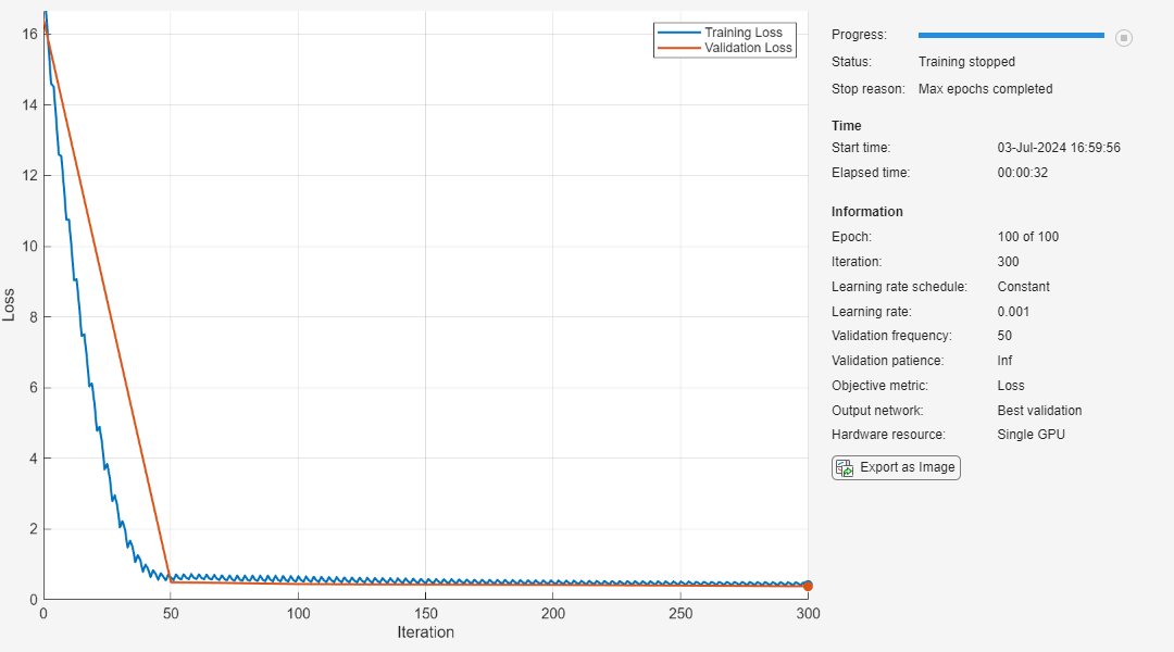
Set the training options.

Train for 100 epochs using the Adam optimizer.
Set the learning rate schedule to "piecewise".
Specify the validation data.
To prevent overfitting, set L2Regularization to 0.1.
Set the InputDataFormats to "CTB" because the training data contains features in the first dimension, time-series sequences in the second dimension, and the batches of the data in the third dimension.
Return the network with the best validation loss.
Turn on the training plot. Turn off the command line output.

options = trainingOptions("adam", ...
    InputDataFormats="CTB", ...
    MaxEpochs=100, ...
    L2Regularization=0.1, ...
    ValidationData={XValidation, TValidation}, ...
    OutputNetwork="best-validation-loss", ...
    Plots="training-progress", ...
    Verbose=false);

netPruned = trainnet(XTrain,TTrain,netPruned,"mse",options);

Test the fine-tuned pruned network. Compare the RMSE of the fine-tuned pruned and original networks.

rmsePrunedNetwork = testnet(netPruned,XTest,TTest,"rmse",InputDataFormats="CTB")

rmsePrunedNetwork = 
0.7920

rmseOriginalNetwork

rmseOriginalNetwork = 
0.8072

Compress Network Using Projection

Projection allows you to convert large layers with many learnables to one or more smaller layers with fewer learnable parameters in total.

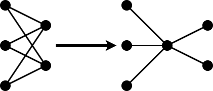
The compressNetworkUsingProjection function applies principal component analysis (PCA) to the training data to identify the subspace of learnable parameters that result in the highest variance in neuron activations.

First, reanalyze the pruned network for compression using Deep Network Designer.

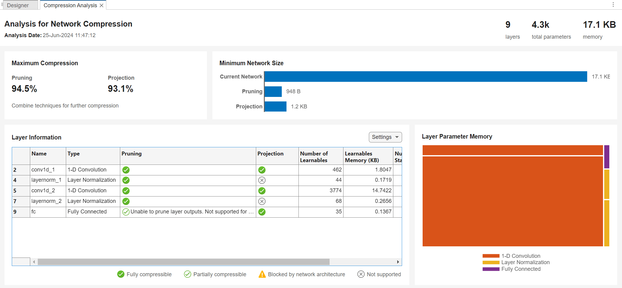
The analysis report shows that you can further compress the network using both pruning and projection. Three layers are fully compressible using projection, conv1d_1, conv1d_2, and fc. For very small layers, such as fc, projection can sometimes increase the number of learnable parameters. Apply projection to the two convolutional layers.

layersToProject = ["conv1d_1" "conv1d_2"];

First, create a mini-batch queue from the training data, as during the pruning step. When performing the PCA step for projection, do not pad sequence data as doing so can negatively impact the analysis. Instead, the mini-batch preprocessing function in this code truncates the sequences to the length of the shortest sequence.

mbqProject = minibatchqueue(cds,2,...
    PartialMiniBatch = "discard", ...
    MiniBatchFcn = @preprocessProjectionMiniBatch, ...
    MiniBatchFormat = ["CTB","BC"]);

function [X,T] = preprocessProjectionMiniBatch(XCell,TCell)
    X = padsequences(XCell,2,Length="shortest",Direction="left");
    T = cell2mat(TCell);
end

Next, use the neuronPCA function to perform PCA.

npca = neuronPCA(netPruned,mbqProject)

Using solver mode "direct".
neuronPCA analyzed 3 layers: "conv1d_1","conv1d_2","fc"

npca = 
  neuronPCA with properties:

                  LayerNames: ["conv1d_1"    "conv1d_2"    "fc"]
      ExplainedVarianceRange: [0 1]
    LearnablesReductionRange: [0 0.9245]
            InputEigenvalues: {[4×1 double]  [18×1 double]  [38×1 double]}
           InputEigenvectors: {[4×4 double]  [18×18 double]  [38×38 double]}
           OutputEigenvalues: {[18×1 double]  [38×1 double]  [1.5035]}
          OutputEigenvectors: {[18×18 double]  [38×38 double]  [1]}

Next, project the network using the compressNetworkUsingProjection function. Specify a learnables reduction goal of 70%. Choosing the learnables reduction goal, or alternatively the explained variance goal, requires empirical analysis and depends on your requirements for network size and accuracy.

If you do not provide the neuronPCA object as an input argument, and instead provide mbqProject directly, the function also performs the PCA step.

netProjected = compressNetworkUsingProjection(netPruned,npca,LearnablesReductionGoal=0.7,LayerNames=layersToProject)

Compressed network has 72.0% fewer learnable parameters.
Projection compressed 2 layers: "conv1d_1","conv1d_2"

netProjected = 
  dlnetwork with properties:

         Layers: [9×1 nnet.cnn.layer.Layer]
    Connections: [8×2 table]
     Learnables: [16×3 table]
          State: [0×3 table]
     InputNames: {'sequenceinput'}
    OutputNames: {'fc'}
    Initialized: 1

  View summary with summary.

Analyze the projected network using the analyzeNetwork function. View information about the projected layers.

info = analyzeNetwork(netProjected,Plots="none");
info.LayerInfo(info.LayerInfo.NumLearnables>0,["Name" "Type" "NumLearnables" "LearnablesReduction"])

ans=5×4 table
        Name                 Type             NumLearnables    LearnablesReduction
    _____________    _____________________    _____________    ___________________

    "conv1d_1"       "Projected Layer"             252               0.33333      
    "layernorm_1"    "Layer Normalization"          36                     0      
    "conv1d_2"       "Projected Layer"             713               0.79381      
    "layernorm_2"    "Layer Normalization"          76                     0      
    "fc"             "Fully Connected"              39                     0

Test the projected network. Compare the RMSE of the projected and original networks.

testnet(netProjected,XTest,TTest,"rmse",InputDataFormats="CTB")

ans = 
0.8704

rmseOriginalNetwork

rmseOriginalNetwork = 
0.8072

Retrain Projected Network

Use the trainnet function to retrain the network for several epochs and regain some of the lost accuracy.

netProjected = trainnet(XTrain,TTrain,netProjected,"mse",options);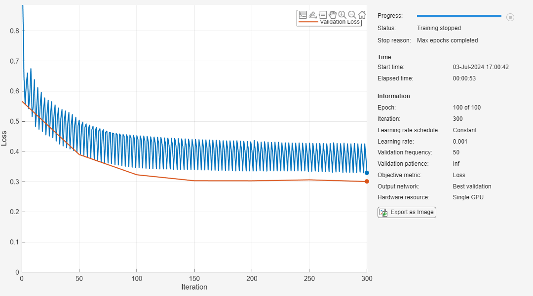

Test the fine-tuned projected network. Compare the RMSE of the fine-tuned projected and original networks.

rmseProjectedNetwork = testnet(netProjected,XTest,TTest,"rmse",InputDataFormats="CTB")

rmseProjectedNetwork = 
0.8028

rmseOriginalNetwork

rmseOriginalNetwork = 
0.8072

Compare Networks

Compare the size and accuracy of the original network, the fine-tuned pruned network, and the fine-tuned pruned and projected network.

infoOriginalNetwork = analyzeNetwork(net,Plots="none");
infoPrunedNetwork = analyzeNetwork(netPruned,Plots="none");
infoProjectedNetwork = analyzeNetwork(netProjected,Plots="none");

numLearnablesOriginalNetwork = infoOriginalNetwork.TotalLearnables;
numLearnablesPrunedNetwork = infoPrunedNetwork.TotalLearnables;
numLearnablesProjectedNetwork = infoProjectedNetwork.TotalLearnables;

figure
tiledlayout("flow")

nexttile
bar([rmseOriginalNetwork rmsePrunedNetwork rmseProjectedNetwork])
xticklabels(["Original" "Pruned" "Pruned and Projected"])
title("RMSE")
ylabel("RMSE")

nexttile
bar([numLearnablesOriginalNetwork numLearnablesPrunedNetwork numLearnablesProjectedNetwork])
xticklabels(["Original" "Pruned" "Pruned and Projected"])
ylabel("Number of Learnables")
title("Number of Learnables")

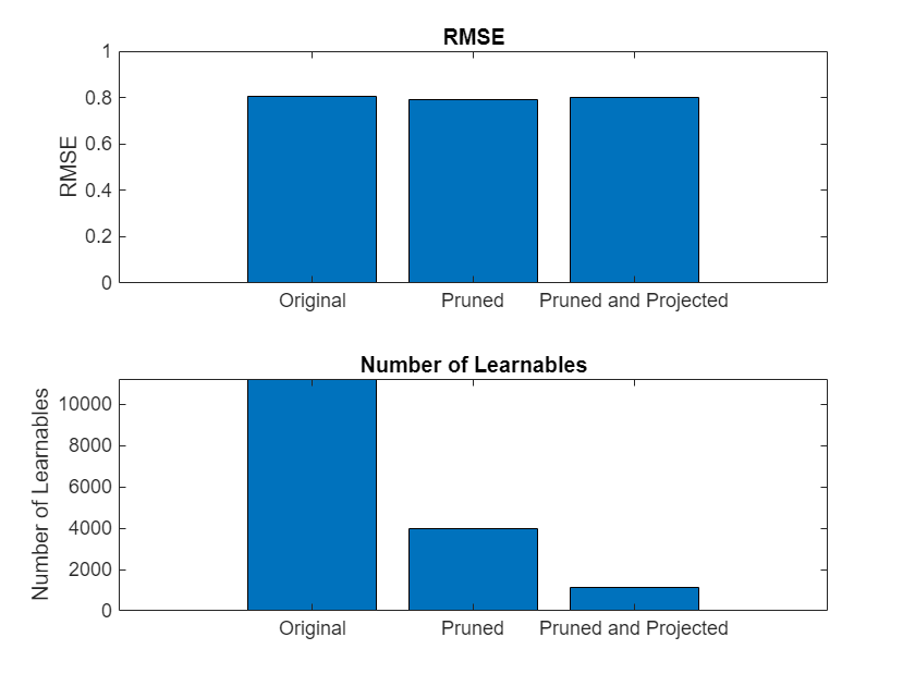
The plot compares the RMSE as well as the number of learnable parameters of the original network, the fine-tuned pruned network, and the fine-tuned pruned and projected network. The number of learnables decreases significantly with each compression step, without any negative impact on the RMSE.

Supporting Function

function [loss, state, gradients, pruningActivations, pruningGradients] = modelLoss(net,X,T)

% Calculate network output for training.
[out, state, pruningActivations] = forward(net,X);

% Calculate loss.
loss = mse(out,T);

% Compute pruning gradients.
gradients = dlgradient(loss,net.Learnables);
pruningGradients = dlgradient(loss,pruningActivations);
end