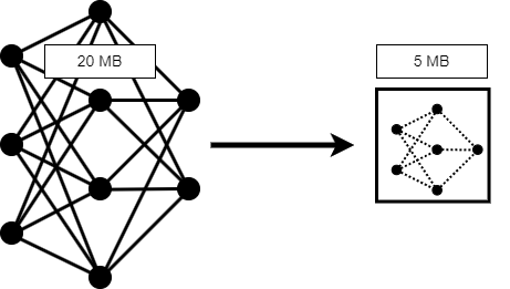
Reduce Memory Footprint of Deep Neural Networks

Neural networks can take up large amounts of memory. If you have a memory requirement for your network, for example because you would like to embed it into a resource-constrained hardware target, then you might need to reduce the size of your model to meet the requirements. This page describes how to use MATLAB^®, and particularly Deep Learning Toolbox Model Quantization Library, to compress your neural network.

Simplified illustration of compression. On the left, there is a sketch of a large neural network with a label indicating it is 20 MB large. An arrow points from this to a second sketch on the right, which shows a smaller model inside a box. A label indicates the smaller network is 5 MB large.

For information on how to speed up neural network training, see Speed Up Deep Neural Network Training. For information on how to improve the accuracy of your network, see Deep Learning Tips and Tricks.

The two main contributors to the memory footprint of a neural network are states and learnable parameters. Layer states contain information calculated during the layer operations to be retained for use in subsequent forward passes of the layer, for example, the cell state and hidden state of LSTM layers. The network learnable parameters contain the features learned by the network, for example, the weights of convolution and fully connected layers.

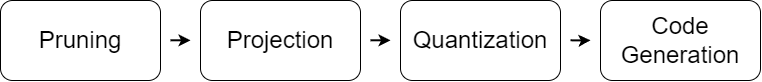
You can compress a network using one of two methods.

Structural compression reduces the number of states and learnable parameters. MATLAB has two structural compression techniques, pruning and projection.
Quantization converts the states and learnable parameters to lower precision data types.

Pruning	Pruning refers to the systematic removal of learnable parameters that have the smallest impact on the predictions of your network.	For an example, see Prune Filters in a Detection Network Using Taylor Scores.
Projection	Projection is a way of converting large layers with many learnables to one or more smaller layers with fewer learnable parameters in total.	For an example, see Compress Neural Network Using Projection.
Quantization	Quantization is a data-type compression technique. You reduce the precision of the parameters in your network, but the amount of parameters and the network architecture stay the same.	For an example, see Quantize Semantic Segmentation Network and Generate CUDA Code.

You can use any combination of these techniques to reduce the size of your network, depending on the types of layers and overall network architecture. For the best results, first prune, then project, then quantize. Then generate code and embed the network on your hardware target. For optimal results, fine-tune your network after each step.

Diagram of suggested compression workflow: first pruning, then projection, then quantization, then code generation.

Use the Deep Network Designer app to analyze your network for memory reduction using compression techniques. Open your network in Deep Network Designer. Then, click Analyze for compression. This feature requires Deep Learning Toolbox™ Model Quantization Library.

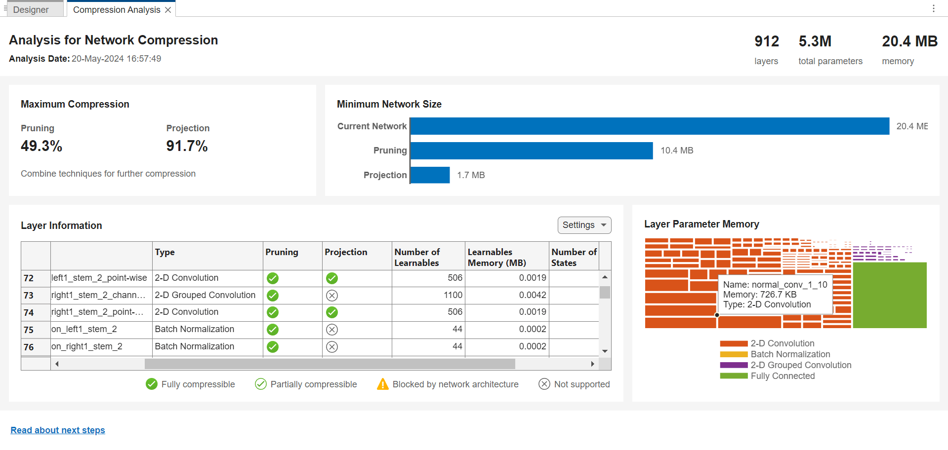
Screenshot of compression analysis report in Deep Network Designer.

The compression analysis report shows information about:

Maximum possible memory reduction
Pruning and projection support
Effect of the network architecture on the ability to prune individual layers
Layer memory

Use the compression analysis report to decide which technique to use to compress your network.

Structural Compression

Structural compression reduces the size of your network by reducing the number of states and learnable parameters. MATLAB has two structural compression techniques, pruning and projection.

Pruning

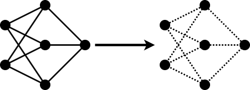
Pruning a neural network means removing the least important parameters to reduce the size of the network while preserving the quality of its predictions.

You can measure the importance of a set of parameters by the change in loss after removal of the parameters from the network. If the loss changes significantly, then the parameters are important. If the loss does not change significantly, then the parameters are not important and can be pruned.

When you have a large number of parameters in your network, you cannot calculate the change in loss for all possible combinations of parameters. Instead, apply an iterative workflow.

Use an approximation to find and remove the least important parameter, or the n least important parameters.
Fine-tune the new, smaller network by retraining it for a couple of iterations.
Repeat steps 1 and 2 until you reach your desired memory reduction or until you cannot recover the accuracy drop via fine-tuning.

One option for the approximation in step 1 is to calculate the Taylor expansion of the loss as a function of the individual network parameters. This method is called Taylor pruning.

For some types of layers, including convolutional layers, removing a parameter is equivalent to setting it to zero. In this case, the change in loss resulting from pruning a parameter θ can be expressed as follows.

$| Δ loss (X, θ) | = | loss (X, θ = 0) - loss (X, θ) | .$

Here, X is the training data of your network.

Calculate the Taylor expansion of the loss as a function of the parameter θ to first order.

$loss (X, θ) = loss (X, θ = 0) + \frac{δ loss}{δ θ} θ .$

Then, you can express the change of loss as a function of the gradient of the loss with respect to the parameter θ.

$| Δ loss (X, θ) | = | \frac{δ loss}{δ θ} θ | .$

You already calculate this gradient during training for backpropagation. You can reuse the same calculation to calculate the gradient for Taylor pruning.

In MATLAB, you can perform Taylor pruning by using a taylorPrunableNetwork object. Implement the iterative pruning process in a custom training loop. Calculate the importance of the learnable parameters using the updateScore function. Remove the n least important learnable parameters using the updatePrunables function. For an example of this workflow, see Prune Image Classification Network Using Taylor Scores.

Pruning using taylorPrunableNetwork objects removes filters from convolutional layers. Pruning convolutional filters can also reduce the number of learnable parameters in downstream layers, for example, batchNormalizationLayer and fullyConnectedLayer objects.

For an example of how to use Taylor pruning on an image classification network in MATLAB, see Prune Image Classification Network Using Taylor Scores. For an example of how to use Taylor pruning on a YOLO v3 object detection model and embed the resulting model onto a Raspberry Pi^®, see Prune Filters in a Detection Network Using Taylor Scores.

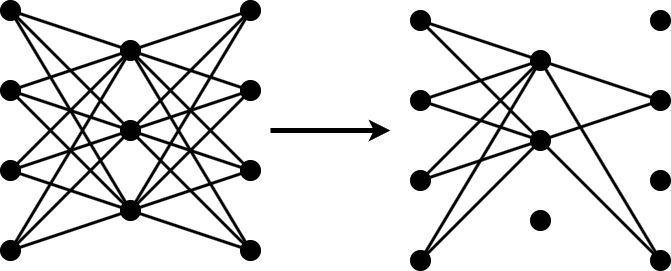
Projection

Projection is a layer-wise compression technique that replaces a large layer with one or more layers with a smaller total number of parameters.

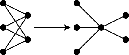
In neural networks, data is usually expressed as a high-dimensional vector. Not all of the dimensions are equally important for the task you are solving. Often, a small subset of elements accounts for a large amount of the variance in the output.

Principal-component analysis (PCA) allows you to express your data in a basis of dimensions sorted by importance. The first element accounts for the largest part of variance, the second for the second-largest part, and the last element for the smallest amount of variance.

Neural network projection uses PCA to reduce the size of a network layer in the following way.

Use PCA to identify the subspace of learnable parameters that result in the highest variance in neuron activations by analyzing the network activations using a data set representative of the training data.
Project the layer input onto the lower-dimensional space spanned by the N most important directions.
Perform the layer operation within the lower-dimensional space.
Return to the higher-dimensional space by appending the required number of zeros to the end of the output and rotate back into the original basis.

In MATLAB, project your neural network using the compressNetworkUsingProjection function. The compressNetworkUsingProjection function performs PCA automatically.

If you want to project the same network several times, for example, to explore different levels of compression, then perform PCA separately using the neuronPCA function. You can then pass the output to the compressNetworkUsingProjection function as an optional input argument.

After projection, retrain your model to regain some or all of the accuracy lost during the projection step.

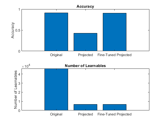
For an example of projection of a sequence classification network, see Compress Neural Network Using Projection. For an example of projection of a network as part of an overarching workflow to estimate battery states of charge, see Evaluate Code Generation Inference Time of Compressed Deep Neural Network.

Quantization

Quantization is a compression technique that does not impact the network architecture, and instead reduces the precision of the learnable parameters. In Deep Learning Toolbox, by default, network parameters are stored in single precision. The Deep Learning Toolbox Model Quantization Library support package allows you to deploy your network with parameters stored as reduced precision types.

The quantization workflow consists of two steps.

Find the dynamic ranges of the parameters in your network. To do so, exercise your network with sample data that is representative of your training data. Extract the minimum and maximum values of the weights and biases in each convolution and fully connected layer. Extract the minimum and maximum values of the activations in all other layers of your network.
In each layer, convert the parameters to integers representing the dynamic range calculated in the previous step.

To quantize deep learning models in MATLAB, you can use either the dlquantizer function or the Deep Network Quantizer app.

Command Line Workflow

At the command line, start by creating a dlquantizer object. Next, use the calibrate function to determine the dynamic ranges of the layer parameters. Make sure the data you pass to the calibrate function is representative of your training data.

Next, you can optionally simulate quantization using the quantize function. This function allows you to test the output of your quantized network independent of your hardware target. Use the quantizationDetails function to display details of the quantization, such as a list of quantized layers, the target library, and the quantized learnable parameters.

You can also use the estimateNetworkMetrics function to estimate the effects of quantization specific layers of your neural network. This function estimates metrics for learnable layers, which have weights and biases, in the network. Estimated metrics are provided for the following supported layers.

You can also use the prepareNetwork function to prepare your network for quantization. This function modifies the neural network to improve accuracy and avoid error conditions in the quantization workflow. These modifications include layer fusion, equalization of layer parameters, replacement of unsupported layers, and conversion of DAGNetwork and SeriesNetwork objects to a dlnetwork object.

Once you are satisfied with your network, validate and quantize your network using the validate function. To choose quantization options, such as the execution environment, use the dlquantizationOptions function. Then, deploy your network to your hardware target.

For information on how to quantize neural networks for different execution environments using the command line, see these examples.

Quantize Semantic Segmentation Network and Generate CUDA Code
Classify Images on FPGA by Using Quantized GoogLeNet Network (Deep Learning HDL Toolbox)
Generate INT8 Code for Deep Learning Network on Raspberry Pi (MATLAB Coder)

Deep Network Quantizer App

You can also use the Deep Network Quantizer app to achieve the quantization workflow. To open the app from the MATLAB command prompt, enter deepNetworkQuantizer.

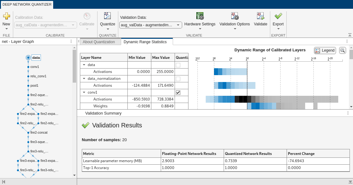
Screenshot of Deep Network Quantizer app.

For information on how to use Deep Network Quantizer to quantize neural networks for different execution environments, see these examples.

Further Information

For more information on quantization, see Quantization of Deep Neural Networks. For information on Quantization Workflow Prerequisites in Deep Learning Toolbox, see Quantization Workflow Prerequisites. For information on how to preprocess data for quantization, see Prepare Data for Quantizing Networks.

Compatibility Considerations

Layers Compatible with Pruning and Projection

Layer	Pruning	Projection
`convolution1dLayer`	Supported	Supported
`convolution2dLayer`	Supported	Supported
`batchNormalizationLayer`	Partially supported. The size of a `batchNormalizationLayer` can reduce if an upstream layer is pruned.	Not supported
`layerNormalizationLayer`	Partially supported. The size of a `layerNormalizationLayer` can reduce if an upstream layer is pruned.	Not supported
`fullyConnectedLayer`	Partially supported. The size of a `fullyConnectedLayer` can reduce if an upstream layer is pruned.	Supported
`groupedConvolution2dLayer`	Partially supported. The size of a `groupedConvolution2dLayer` can reduce if an upstream layer is pruned.	Not supported
`TransposedConvolution1DLayer`	Partially supported. The size of a `TransposedConvolution1dLayer` can reduce if an upstream layer is pruned.	Not supported
`TransposedConvolution2DLayer`	Partially supported. The size of a `TransposedConvolution2dLayer` can reduce if an upstream layer is pruned.	Not supported
`lstmLayer`	Not supported	Supported
`gruLayer`	Not supported	Supported

You can also analyze your network for compatibility with pruning and projection using Deep Network Designer.

The networks and layers that support quantization depend on the target execution environment. For execution on GPU, see Supported Networks, Layers, and Classes (GPU Coder). For execution on FPGA, see Supported Networks, Layers, Boards, and Tools (Deep Learning HDL Toolbox). For execution on CPU or in MATLAB, see Networks and Layers Supported for Code Generation (MATLAB Coder).

Other Techniques

The techniques described in the previous section are part of the Deep Learning Toolbox Model Quantization Library. There are several other compression techniques in MATLAB.

Knowledge Distillation

In knowledge distillation, use a large and accurate teacher network to teach a smaller student network to make accurate predictions [2]. This technique allows you to design a small network to fit your memory requirements. For an example of knowledge distillation in MATLAB, see Train Smaller Neural Network Using Knowledge Distillation.

Quantization Using NVIDIA TensorRT Library (GPU Coder)

You can generate code for 8-bit integer prediction using the NVIDIA TensorRT library. For an example, see Deep Learning Prediction with NVIDIA TensorRT Library.

Quantization Using `bfloat16` Code (MATLAB Coder)

The brain floating-point (bfloat16) format is a truncated version of the single-precision floating-point format. It only occupies 16 bits in computer memory. bfloat16 preserves approximately the same number range as single-precision floating-point by retaining the same number of exponent bits. For information on how to generate and deploy bfloat16 code for deep learning networks, see Generate bfloat16 Code for Deep Learning Networks (MATLAB Coder).

Sparsity

You can use sparsity to prune a network using a custom importance metric. Identify the least important parameters, set them to zero, and store the resulting weights matrices as sparse matrices.

For an example of pruning by using magnitude scores and synaptic flow scores, see Parameter Pruning and Quantization of Image Classification Network. Both of these metrics are data-free importance estimation techniques.

Fixed-Point Designer

To use reduced precision types to optimize general algorithms for embedded hardware, use Fixed-Point Designer™. For more information, see Benefits of Fixed-Point Hardware (Fixed-Point Designer).

References

[1] Molchanov, Pavlo, Stephen Tyree, Tero Karras, Timo Aila, and Jan Kautz. "Pruning Convolutional Neural Networks for Resource Efficient Inference." Preprint, submitted June 8, 2017. https://arxiv.org/abs/1611.06440.

[2] Hinton, Geoffrey, Oriol Vinyals, and Jeff Dean. “Distilling the Knowledge in a Neural Network.” Preprint, submitted March 9, 2015. https://arxiv.org/abs/1503.02531.

[3] Google Cloud Blog. “BFloat16: The Secret to High Performance on Cloud TPUs.” Accessed January 26, 2023. https://cloud.google.com/blog/products/ai-machine-learning/bfloat16-the-secret-to-high-performance-on-cloud-tpus.