使用贝叶斯优化进行深度学习
此示例说明如何将贝叶斯优化应用于深度学习并找到卷积神经网络的最优网络超参数和训练选项。
要训练深度神经网络,您必须指定神经网络架构以及训练算法的选项。选择和调整这些超参数可能很困难并且需要时间。贝叶斯优化是一种非常适合对分类模型和回归模型的超参数进行优化的算法。您可以使用贝叶斯优化来对不可微分、不连续且计算耗时的函数进行优化。该算法在内部维护目标函数的高斯过程模型,并使用目标函数计算来训练此模型。
以下示例演示如何:
下载并准备 CIFAR-10 数据集以进行网络训练。此数据集是一个广泛用于测试图像分类模型的数据集。
指定要使用贝叶斯优化进行优化的变量。这些变量是训练算法的选项,以及网络架构本身的参数。
定义目标函数,该函数将优化变量的值作为输入,指定网络架构和训练选项,训练和验证网络,并将经过训练的网络保存到磁盘。目标函数在此脚本的末尾定义。
通过最大程度地减小对验证集的分类误差来执行贝叶斯优化。
从磁盘加载最佳网络并基于测试集对其进行评估。
您也可以使用贝叶斯优化在Experiment Manager中找到最佳训练选项。有关详细信息,请参阅Tune Experiment Hyperparameters by Using Bayesian Optimization。
准备数据
下载 CIFAR-10 数据集 [1]。该数据集包含 60,000 个图像,每个图像的大小为 32×32,并具有三个颜色通道 (RGB)。整个数据集的大小为 175 MB。下载过程可能需要一些时间,具体取决于您的 Internet 连接情况。
datadir = tempdir;
downloadCIFARData(datadir);
加载 CIFAR-10 数据集,用作训练图像和标签以及测试图像和标签。要启用网络验证,请将 5000 个测试图像用于验证。
[XTrain,YTrain,XTest,YTest] = loadCIFARData(datadir);

idx = randperm(numel(YTest),5000);
XValidation = XTest(:,:,:,idx);
XTest(:,:,:,idx) = [];
YValidation = YTest(idx);
YTest(idx) = [];
您可以使用以下代码显示训练图像的样本。
figure;
idx = randperm(numel(YTrain),20);
for i = 1:numel(idx)
    subplot(4,5,i);
    imshow(XTrain(:,:,:,idx(i)));
end
选择要优化的变量
选择要使用贝叶斯优化对哪些变量进行优化,并指定搜索范围。此外,指定变量是否为整数以及是否搜索对数空间中的区间。优化以下变量:
网络部分深度。此参数控制网络的深度。网络有三个部分,每个部分都有
SectionDepth个相同的卷积层。因此卷积层的总数为3*SectionDepth。脚本稍后部分中的目标函数在每个层中采用与1/sqrt(SectionDepth)成比例的卷积滤波器数量。因此,对于不同的部分深度,每次迭代的参数数量和所需的计算量大致相同。初始化学习率。最佳学习率取决于您的数据以及您正在训练的网络。
随机梯度下降动量。动量在当前参数更新中包含一个与前一次迭代中的更新成比例的贡献,从而在更新中增加惯性。这会使参数更新更加平滑,并减少随机梯度下降固有的噪声。
L2 正则化强度。使用正则化以防止过拟合。搜索正则化强度的空间以查找良好的值。数据增强和批量归一化也有助于正则化网络。
optimVars = [
    optimizableVariable('SectionDepth',[1 3],'Type','integer')
    optimizableVariable('InitialLearnRate',[1e-2 1],'Transform','log')
    optimizableVariable('Momentum',[0.8 0.98])
    optimizableVariable('L2Regularization',[1e-10 1e-2],'Transform','log')];
执行贝叶斯优化
使用训练数据和验证数据作为输入,为贝叶斯优化器创建目标函数。目标函数训练一个卷积神经网络并返回对验证集的分类误差。该函数在此脚本的末尾定义。由于 bayesopt 使用基于验证集的误差率来选择最佳模型,因此最终网络可能会对验证集过拟合。随后基于独立测试集测试最终选择的模型,以估计泛化误差。
ObjFcn = makeObjFcn(XTrain,YTrain,XValidation,YValidation);
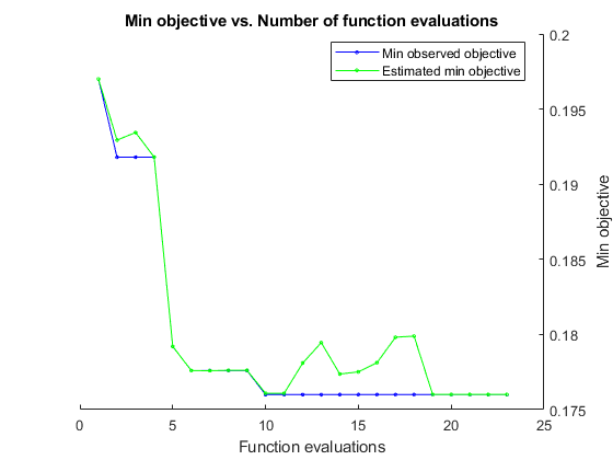
通过最大程度地减小对验证集的分类误差来执行贝叶斯优化。以秒为单位指定总优化时间。为了最好地利用贝叶斯优化的能力,您应该执行至少 30 次对象函数评估。要在多个 GPU 上并行训练网络,请将 'UseParallel' 值设置为 true。如果您有一个 GPU 并将 'UseParallel' 值设置为 true,则所有工作单元将共用该 GPU,这不仅无法加速训练,而且会增加 GPU 耗尽内存的几率。
每个网络完成训练后,bayesopt 将结果显示到命令行窗口。然后,bayesopt 函数返回 BayesObject.UserDataTrace 中的文件名。目标函数将经过训练的网络保存到磁盘,并将文件名返回到 bayesopt。
BayesObject = bayesopt(ObjFcn,optimVars, ...
    'MaxTime',14*60*60, ...
    'IsObjectiveDeterministic',false, ...
    'UseParallel',false);
|===================================================================================================================================|
| Iter | Eval   | Objective   | Objective   | BestSoFar   | BestSoFar   | SectionDepth | InitialLearn-|     Momentum | L2Regulariza-|
|      | result |             | runtime     | (observed)  | (estim.)    |              | Rate         |              | tion         |
|===================================================================================================================================|
|    1 | Best   |       0.197 |      955.69 |       0.197 |       0.197 |            3 |      0.61856 |      0.80624 |   0.00035179 |
| 2 | Best | 0.1918 | 790.38 | 0.1918 | 0.19293 | 2 | 0.074118 | 0.91031 | 2.7229e-09 |
| 3 | Accept | 0.2438 | 660.29 | 0.1918 | 0.19344 | 1 | 0.051153 | 0.90911 | 0.00043113 |
| 4 | Accept | 0.208 | 672.81 | 0.1918 | 0.1918 | 1 | 0.70138 | 0.81923 | 3.7783e-08 |
| 5 | Best | 0.1792 | 844.07 | 0.1792 | 0.17921 | 2 | 0.65156 | 0.93783 | 3.3663e-10 |
| 6 | Best | 0.1776 | 851.49 | 0.1776 | 0.17759 | 2 | 0.23619 | 0.91932 | 1.0007e-10 |
| 7 | Accept | 0.2232 | 883.5 | 0.1776 | 0.17759 | 2 | 0.011147 | 0.91526 | 0.0099842 |
| 8 | Accept | 0.2508 | 822.65 | 0.1776 | 0.17762 | 1 | 0.023919 | 0.91048 | 1.0002e-10 |
| 9 | Accept | 0.1974 | 1947.6 | 0.1776 | 0.17761 | 3 | 0.010017 | 0.97683 | 5.4603e-10 |
| 10 | Best | 0.176 | 1938.4 | 0.176 | 0.17608 | 2 | 0.3526 | 0.82381 | 1.4244e-07 |
| 11 | Accept | 0.1914 | 2874.4 | 0.176 | 0.17608 | 3 | 0.079847 | 0.86801 | 9.7335e-07 |
| 12 | Accept | 0.181 | 2578 | 0.176 | 0.17809 | 2 | 0.35141 | 0.80202 | 4.5634e-08 |
| 13 | Accept | 0.1838 | 2410.8 | 0.176 | 0.17946 | 2 | 0.39508 | 0.95968 | 9.3856e-06 |
| 14 | Accept | 0.1786 | 2490.6 | 0.176 | 0.17737 | 2 | 0.44857 | 0.91827 | 1.0939e-10 |
| 15 | Accept | 0.1776 | 2668 | 0.176 | 0.17751 | 2 | 0.95793 | 0.85503 | 1.0222e-05 |
| 16 | Accept | 0.1824 | 3059.8 | 0.176 | 0.17812 | 2 | 0.41142 | 0.86931 | 1.447e-06 |
| 17 | Accept | 0.1894 | 3091.5 | 0.176 | 0.17982 | 2 | 0.97051 | 0.80284 | 1.5836e-10 |
| 18 | Accept | 0.217 | 2794.5 | 0.176 | 0.17989 | 1 | 0.2464 | 0.84428 | 4.4938e-06 |
| 19 | Accept | 0.2358 | 4054.2 | 0.176 | 0.17601 | 3 | 0.22843 | 0.9454 | 0.00098248 |
| 20 | Accept | 0.2216 | 4411.7 | 0.176 | 0.17601 | 3 | 0.010847 | 0.82288 | 2.4756e-08 |
|===================================================================================================================================|
| Iter | Eval   | Objective   | Objective   | BestSoFar   | BestSoFar   | SectionDepth | InitialLearn-|     Momentum | L2Regulariza-|
|      | result |             | runtime     | (observed)  | (estim.)    |              | Rate         |              | tion         |
|===================================================================================================================================|
|   21 | Accept |      0.2038 |      3906.4 |       0.176 |     0.17601 |            2 |      0.09885 |      0.81541 |    0.0021184 |
| 22 | Accept | 0.2492 | 4103.4 | 0.176 | 0.17601 | 2 | 0.52313 | 0.83139 | 0.0016269 |
| 23 | Accept | 0.1814 | 4240.5 | 0.176 | 0.17601 | 2 | 0.29506 | 0.84061 | 6.0203e-10 |
__________________________________________________________
Optimization completed.
MaxTime of 50400 seconds reached.
Total function evaluations: 23
Total elapsed time: 53088.5123 seconds
Total objective function evaluation time: 53050.7026

Best observed feasible point:
    SectionDepth    InitialLearnRate    Momentum    L2Regularization
    ____________    ________________    ________    ________________

         2               0.3526         0.82381        1.4244e-07

Observed objective function value = 0.176
Estimated objective function value = 0.17601
Function evaluation time = 1938.4483

Best estimated feasible point (according to models):
    SectionDepth    InitialLearnRate    Momentum    L2Regularization
    ____________    ________________    ________    ________________

         2               0.3526         0.82381        1.4244e-07

Estimated objective function value = 0.17601
Estimated function evaluation time = 1898.2641
评估最终网络
加载在优化中找到的最佳网络及其验证准确度。
bestIdx = BayesObject.IndexOfMinimumTrace(end);
fileName = BayesObject.UserDataTrace{bestIdx};
savedStruct = load(fileName);
valError = savedStruct.valError
valError = 0.1760
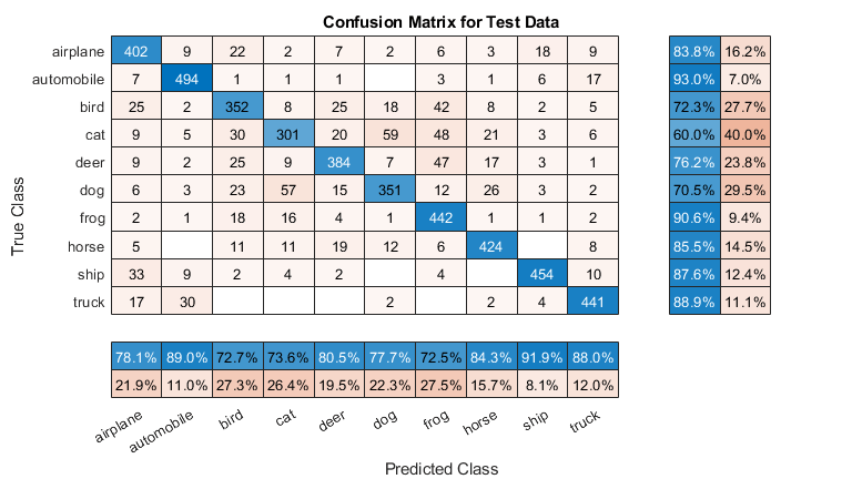
预测测试集的标签并计算测试误差。将测试集中每个图像的分类视为具有一定成功概率的独立事件,这意味着分类错误的图像数量遵循二项分布。使用这种方法来计算标准误差 (testErrorSE) 和泛化误差率的约 95% 置信区间 (testError95CI)。此方法通常称为 Wald 方法。bayesopt 使用验证集确定最佳网络,而不对网络使用测试集。因此,测试误差可能高于验证误差。
[YPredicted,probs] = classify(savedStruct.trainedNet,XTest);
testError = 1 - mean(YPredicted == YTest)
testError = 0.1910
NTest = numel(YTest);
testErrorSE = sqrt(testError*(1-testError)/NTest);
testError95CI = [testError - 1.96*testErrorSE, testError + 1.96*testErrorSE]
testError95CI = 1×2

    0.1801    0.2019
绘制测试数据的混淆矩阵。使用列汇总和行汇总显示每个类的准确率和召回率。
figure('Units','normalized','Position',[0.2 0.2 0.4 0.4]);
cm = confusionchart(YTest,YPredicted);
cm.Title = 'Confusion Matrix for Test Data';
cm.ColumnSummary = 'column-normalized';
cm.RowSummary = 'row-normalized';
您可以使用以下代码显示一些测试图像以及它们的预测类和这些类的概率。
figure
idx = randperm(numel(YTest),9);
for i = 1:numel(idx)
    subplot(3,3,i)
    imshow(XTest(:,:,:,idx(i)));
    prob = num2str(100*max(probs(idx(i),:)),3);
    predClass = char(YPredicted(idx(i)));
    label = [predClass,', ',prob,'%'];
    title(label)
end
优化的目标函数
定义优化的目标函数。此函数执行以下步骤:
将优化变量的值作为输入。
bayesopt使用某个表中的优化变量的当前值调用目标函数,该表的每个列名等于变量名称。例如,网络部分深度的当前值为optVars.SectionDepth。定义网络架构和训练选项。
训练并验证网络。
将经过训练的网络、验证误差和训练选项保存到磁盘。
返回已保存网络的验证误差和文件名。
function ObjFcn = makeObjFcn(XTrain,YTrain,XValidation,YValidation)
ObjFcn = @valErrorFun;
    function [valError,cons,fileName] = valErrorFun(optVars)
定义卷积神经网络架构。
对卷积层进行填充,使空间输出大小始终与输入大小相同。
每次使用最大池化层将空间维度下采样一半时,将滤波器数量增加一倍。这样做可确保每个卷积层所需的计算量大致相同。
选择与
1/sqrt(SectionDepth)成比例的滤波器数量,使不同深度的网络具有大致相同的参数个数,并且每次迭代所需的计算量大致相同。要增加网络参数的个数和网络整体灵活性,请增大numF值。要训练更深的网络,请更改SectionDepth变量的范围。使用
convBlock(filterSize,numFilters,numConvLayers)创建numConvLayers卷积层模块,其中每个层都有指定的filterSize和numFilters滤波器,并且每个层都后接一个批量归一化层和一个 ReLU 层。convBlock函数在此示例的末尾定义。
        imageSize = [32 32 3];
        numClasses = numel(unique(YTrain));
        numF = round(16/sqrt(optVars.SectionDepth));
        layers = [
            imageInputLayer(imageSize)

            % The spatial input and output sizes of these convolutional
            % layers are 32-by-32, and the following max pooling layer
            % reduces this to 16-by-16.
            convBlock(3,numF,optVars.SectionDepth)
            maxPooling2dLayer(3,'Stride',2,'Padding','same')

            % The spatial input and output sizes of these convolutional
            % layers are 16-by-16, and the following max pooling layer
            % reduces this to 8-by-8.
            convBlock(3,2*numF,optVars.SectionDepth)
            maxPooling2dLayer(3,'Stride',2,'Padding','same')

            % The spatial input and output sizes of these convolutional
            % layers are 8-by-8. The global average pooling layer averages
            % over the 8-by-8 inputs, giving an output of size
            % 1-by-1-by-4*initialNumFilters. With a global average
            % pooling layer, the final classification output is only
            % sensitive to the total amount of each feature present in the
            % input image, but insensitive to the spatial positions of the
            % features.
            convBlock(3,4*numF,optVars.SectionDepth)
            averagePooling2dLayer(8)

            % Add the fully connected layer and the final softmax and
            % classification layers.
            fullyConnectedLayer(numClasses)
            softmaxLayer
            classificationLayer];
指定网络训练的选项。优化初始学习率、SGD 动量和 L2 正则化强度。
指定验证数据并选择 'ValidationFrequency' 值,使 trainNetwork 每轮训练都验证一次网络。进行固定轮数的训练,并在最后几轮将学习率降低为原来的十分之一。这会减少参数更新的噪声,并使网络参数稳定下来,更接近于损失函数的最小值。
        miniBatchSize = 256;
        validationFrequency = floor(numel(YTrain)/miniBatchSize);
        options = trainingOptions('sgdm', ...
            'InitialLearnRate',optVars.InitialLearnRate, ...
            'Momentum',optVars.Momentum, ...
            'MaxEpochs',60, ...
            'LearnRateSchedule','piecewise', ...
            'LearnRateDropPeriod',40, ...
            'LearnRateDropFactor',0.1, ...
            'MiniBatchSize',miniBatchSize, ...
            'L2Regularization',optVars.L2Regularization, ...
            'Shuffle','every-epoch', ...
            'Verbose',false, ...
            'Plots','training-progress', ...
            'ValidationData',{XValidation,YValidation}, ...
            'ValidationFrequency',validationFrequency);
使用数据增强沿垂直轴随机翻转训练图像,并在水平方向和垂直方向上将图像随机平移最多四个像素。数据增强有助于防止网络过拟合和记忆训练图像的具体细节。
        pixelRange = [-4 4];
        imageAugmenter = imageDataAugmenter( ...
            'RandXReflection',true, ...
            'RandXTranslation',pixelRange, ...
            'RandYTranslation',pixelRange);
        datasource = augmentedImageDatastore(imageSize,XTrain,YTrain,'DataAugmentation',imageAugmenter);
训练网络并在训练过程中绘制训练进度。训练结束后关闭所有训练图。
        trainedNet = trainNetwork(datasource,layers,options);
        close(findall(groot,'Tag','NNET_CNN_TRAININGPLOT_UIFIGURE'))
基于验证集评估经过训练的网络,计算预测的图像标签,并计算基于验证数据的误差率。
        YPredicted = classify(trainedNet,XValidation);
        valError = 1 - mean(YPredicted == YValidation);
创建包含验证误差的文件名,并将网络、验证误差和训练选项保存到磁盘。目标函数返回 fileName 作为输出参量,bayesopt 返回 BayesObject.UserDataTrace 中的所有文件名。额外的必需输出参量 cons 指定变量之间的约束。没有变量约束。
        fileName = num2str(valError) + ".mat";
        save(fileName,'trainedNet','valError','options')
        cons = [];

    end
end
convBlock 函数创建 numConvLayers 卷积层模块,其中每个层都有指定的 filterSize 和 numFilters 滤波器,并且每个层都后接一个批量归一化层和一个 ReLU 层。
function layers = convBlock(filterSize,numFilters,numConvLayers)
layers = [
    convolution2dLayer(filterSize,numFilters,'Padding','same')
    batchNormalizationLayer
    reluLayer];
layers = repmat(layers,numConvLayers,1);
end
参考
[1] Krizhevsky, Alex. "Learning multiple layers of features from tiny images." (2009). https://www.cs.toronto.edu/~kriz/learning-features-2009-TR.pdf
另请参阅
试验管理器 | trainnet | trainingOptions | dlnetwork | bayesopt (Statistics and Machine Learning Toolbox)