Generate Images in Specific Class Using Guided Diffusion
This example shows how to generate new images using a guided diffusion model.
A diffusion model learns to generate images through a training process that involves iteratively adding noise to a clear image, and then attempting to reconstruct the original clear image from the noisy version. The model predicts the added noise and subtracts it from the image, gradually removing the noise and restoring the original clear image. The network generates images that resembles a random part of the training image distribution.
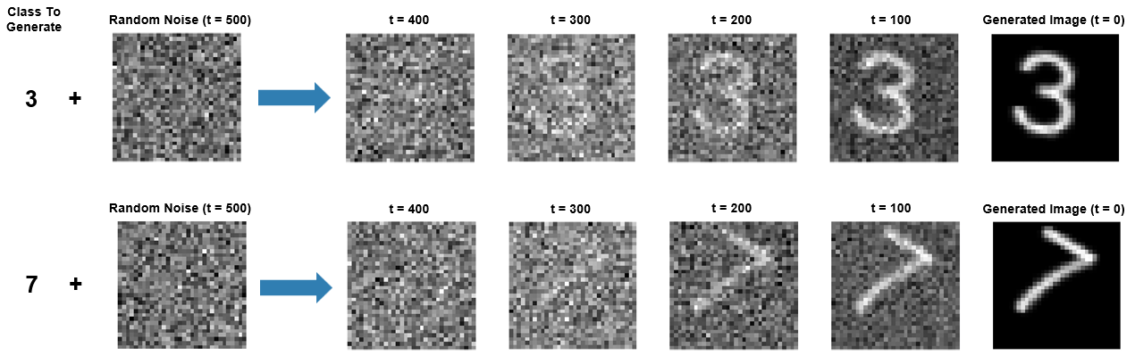
To generate images that belong to a particular class, you can provide class labels as input to the network during training. Once you have trained the network, you can use it to generate new images by starting from random noise and gradually removing the noise that the network predicts, and optionally specifying a class that the image should belong to. Networks that can generate images that belong to a particular class are referred to as conditional or guided diffusion models.
This example trains and generates images using a classifier-free, guided diffusion model. For an example showing how to train and generate images using an unconditional (or nonguided) diffusion model, see Generate Images Using Diffusion.
Load Data
Load the digits data as an image datastore using the imageDatastore function and specify the folder containing the image data.
dataFolder = fullfile(tempdir,"DigitsData");
unzip("DigitsData.zip",dataFolder);
imds = imageDatastore(dataFolder,IncludeSubfolders=true,LabelSource="foldernames");
Use an augmented image datastore to resize the images to have size 32-by-32 pixels.
imgSize = [32 32];
audsImds = augmentedImageDatastore(imgSize,imds);
Forward Diffusion Process
The forward diffusion (noising) process iteratively adds Gaussian noise to an image until the result is indistinguishable from random noise. At each noising step , add Gaussian noise using the equation:
where is the th noisy image and is the variance schedule. The variance schedule defines how the model adds noise to the images. In this example, you define a cosine variance schedule of 500 steps created using the cosineSchedule function, defined at the end of this example. A cosine variance schedule adds noise more slowly than a linear schedule, which avoids images being too noisy too early in the noising process [1]. This can make training converge quicker, particularly when the training images are low resolution (64-by-64 pixels or smaller).
numNoiseSteps = 500;
varianceSchedule = cosineSchedule(numNoiseSteps);
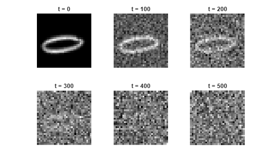
Apply the forward diffusion process on a test image. Extract a single image from the augmented image datastore and rescale it so that the pixel values are in the range [-1 1].
img = read(audsImds);
img = img{1,1};
img = img{:};
img = rescale(img,-1,1);
Use the helper function applyNoiseToImage, defined at the end of this example, to apply increasing amounts of noise to the test image. To display the output at intermediate points, apply numNoiseSteps steps of noise to the image.
Starting from a clear image on the left, the diffusion process adds more noise until the final noising step where the image is indistinguishable from random noise.
figure
tiledlayout
nexttile
imshow(img,[])
title("t = 0");

for i = 1:5
    nexttile
    noise = randn(size(img),like=img);
    noiseStepsToApply = numNoiseSteps/5 * i;
    noisyImg = applyNoiseToImage(img,noise,noiseStepsToApply,varianceSchedule);

    % Extract the data from the dlarray.
    noisyImg = extractdata(noisyImg);
    imshow(noisyImg,[])
    title("t = " + noiseStepsToApply);
end
If you know the added noise at each step, you can reverse the process exactly to recreate the original clear image. Then, if you know the exact statistical distribution of the images, you can perform the reverse process for any random noise to create an image drawn from the training data distribution.
The exact statistical distribution of the dataset is too complicated to compute analytically. However, this example shows how you can train a deep learning network to approximate it. Once you have trained the network, you can use it to generate new images by starting from random noise and successively removing the added noise that the network predicts (denoising).
Define Network
The network architecture is based on the network used in [2] and implements classifier-free guidance as described in [3]. The guidance is referred to as classifier-free because you do not need to train a separate image classifier network.
The network takes three inputs: an image input, a class label, and a scalar feature input representing the number of noise steps added to the image. The network outputs a single image representing the noise that the model predicts has been added to the image.
The network is built around two types of repeating units:
Residual blocks
Attention blocks
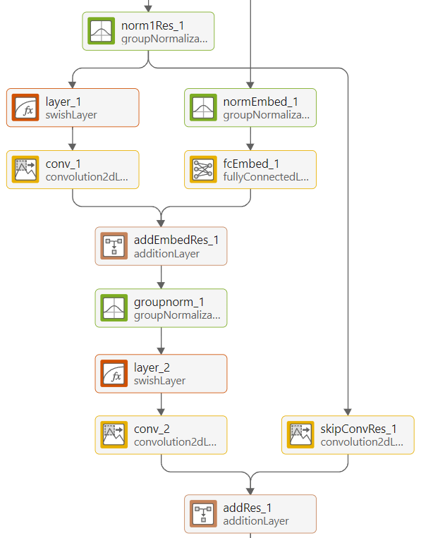
The residual blocks perform convolution operations with skip connections.
The attention blocks perform self-attention operations with skip connections.
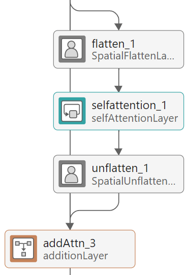
The network has an encoder-decoder structure similar to a U-Net [4]. It repeatedly downsamples an input image to a lower resolution, processes it, and then repeatedly upsamples it to the original size. The network processes the inputs using residual blocks at each resolution. At resolutions of 16-by-16 and 8-by-8 pixels, the network uses attention blocks, which contain self-attention layers, to learn correlations between parts of the input image. To use self-attention layers, the network reshapes the activations using the custom SpatialFlattenLayer so that they have a single spatial dimension. After applying attention, the network reshapes the activations back to 2-D images using the custom SpatialUnflattenLayer. Both layers are included as supporting files with this example.
The network encodes the noise step input using sinusoidal position encoding and adds it to each residual block so that the network can learn to distinguish between different amounts of added noise. The network combines the output of each downsampling residual block with the output of its complementary upsampling residual block using depth concatenation.
The network is conditioned on the image class labels. During training, you pass the one-hot encoded label and provide this to the network. The label passes through a fully-connected network which is then concatenated with the encoded noise step input.
To create the guided diffusion network, use the function createGuidedDiffusionNetwork, attached to this example as a supporting file. This example uses grayscale images, which have one color channel. To train a network on RGB images, change the numInputChannels value to 3.
numInputChannels = 1;
numClasses = numel(unique(imds.Labels));
net = createGuidedDiffusionNetwork(numInputChannels,numClasses);
The full guided diffusion network has 212 layers. To see the full network architecture, use Deep Network Designer.
deepNetworkDesigner(net)
Define Model Loss Function
Create the function modelLoss, listed in the Model Loss Function section of this example. The function takes as input the network, a mini-batch of noisy images with different amounts of noise applied, a mini-batch of noise step values corresponding to the amount of noise added to each image, and the corresponding target noise values.
Specify Training Options
Train with a mini-batch size of 128 for 100 epochs.
miniBatchSize = 128;
numEpochs = 100;
Specify the options for Adam optimization:
A learning rate of 0.0005
A gradient decay factor of 0.9
A squared gradient decay factor of 0.9999
learnRate = 0.0005;
gradientDecayFactor = 0.9;
squaredGradientDecayFactor = 0.9999;
Train Conditioned Model
Train the network to predict the added noise for an image at the specified noise step. The network is trained as described in the Generate Images Using Diffusion example and additionally uses the image labels as input.
Training the network while providing the labels as input allows the network to learn how to remove noise so as to generate images that belong to a specific class (e.g. images that resemble a specific digit). A percentage of the image labels are discarded during and a null class label is used instead. Using some null class labels allows the network to also learn how to generate images that do not belong to a specific class and might resemble any digit.
To train the model, in each epoch, shuffle the training data and loop over the mini-batches. For each mini-batch:
Read the images and labels from the mini-batch queue.
Randomly replace 20% of the image labels with a null label (a vector of zeros).
Choose a random number of noise steps
Nbetween1andnumNoiseSteps.Generate a matrix of random noise the same size as the image and drawn from a standard normal distribution. This is the target that the network learns to predict.
Apply
Niterations of the target noise to the image.
Then, compute the model loss function between the network output and the actual noise added to the images, along with the gradients of the loss function. Update the learnable parameters of the network using gradient descent along the gradients of the loss function.
Training the model is a computationally expensive process that can take hours. To save time while running this example, load a pretrained network by setting doTraining to false. To train the network yourself, set doTraining to true.
doTraining = false;
Use a minibatchqueue object to process and manage the mini-batches of images. In each mini-batch, rescale the images so that the pixel values are in the range [-1 1] using the custom mini-batch preprocessing function preprocessMinibatch, defined at the end of this example.
mbq = minibatchqueue(audsImds, ...
    MiniBatchSize=miniBatchSize, ...
    MiniBatchFcn=@preprocessMiniBatch, ...
    MiniBatchFormat=["SSCB" "CB"], ...
    PartialMiniBatch="discard");
Initialize the parameters for Adam optimization.
averageGrad = [];
averageSqGrad = [];
To track the model performance, use a trainingProgressMonitor object. Calculate the total number of iterations for the monitor.
numObservationsTrain = numel(imds.Files);
numIterationsPerEpoch = ceil(numObservationsTrain/miniBatchSize);
numIterations = numEpochs*numIterationsPerEpoch;
Initialize the TrainingProgressMonitor object. Because the timer starts when you create the monitor object, make sure that you create the object close to the training loop.
if doTraining
    monitor = trainingProgressMonitor(...
        Metrics="Loss", ...
        Info=["Epoch" "Iteration"], ...
        XLabel="Iteration");
end
Train the network.
if doTraining
    iteration = 0;
    epoch = 0;

    while epoch < numEpochs && ~monitor.Stop
        epoch = epoch + 1;
        shuffle(mbq);

        while hasdata(mbq) && ~monitor.Stop
            iteration = iteration + 1;

            [img,labels] = next(mbq);

            % Replace 20% of labels with null label.
            probUnconditional = 0.2;
            labelsToRemoveIdx = randperm(miniBatchSize,round(probUnconditional*miniBatchSize));
            labels(:,labelsToRemoveIdx) = 0;

            % Generate a random noise step.
            noiseStep = dlarray(randi(numNoiseSteps,[1 miniBatchSize],Like=img),"CB");

            % Generate random noise.
            targetNoise = randn(size(img),Like=img);

            % Apply noise to the image.
            noisyImage = applyNoiseToImage(img,targetNoise,noiseStep,varianceSchedule);

            % Compute loss.
            [loss,gradients] = dlfeval(@modelLoss,net,noisyImage,noiseStep,labels,targetNoise);

            % Update model.
            [net,averageGrad,averageSqGrad] = adamupdate(net,gradients,averageGrad,averageSqGrad,iteration, ...
                learnRate,gradientDecayFactor,squaredGradientDecayFactor);

            % Record metrics.
            recordMetrics(monitor,iteration,Loss=loss);
            updateInfo(monitor,Epoch=epoch,Iteration=iteration);
            monitor.Progress = 100 * iteration/numIterations;
        end

        % Every 10 epochs, generate three images in random classes and three images in no class.
        if mod(epoch,10) == 0
            generateAndDisplayImages(net,varianceSchedule,imgSize,numInputChannels,numNoiseSteps + 1,randperm(numClasses,6),[0 0 0 5 5 5],numClasses);
        end
    end
else
    % If doTraining is false, download and extract the pretrained network from the MathWorks website.
    pretrainedNetZipFile = matlab.internal.examples.downloadSupportFile('nnet','data/DigitGenerationModel.zip');
    unzip(pretrainedNetZipFile);
    load("DigitGenerationModel.mat");
end
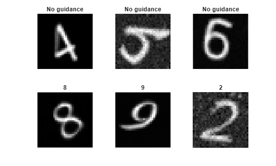
Generate New Images
Use the supporting function generateAndDisplayImages to generate a batch of images using the trained network and display intermediate images after every denoising step to show the denoising process in action.
The function starts with a random image and iterates through the diffusion process in reverse, predicting noise using the network and removing it.
While the forward diffusion process progressively adds more noise in 500 steps, the generateAndDisplayImages function predicts the noise applied by only 15 forward noising steps using a Denoising Diffusion Implicit Model (DDIM) sampling method [5]. This accelerates image generation as the network does not need to make 500 separate predictions to generate each image.
classesToGenerate = randperm(numClasses,6);
guidanceStrength = [0 0 0 10 10 10];
displayFrequency = 1;

figure
generateAndDisplayImages(net,varianceSchedule,imgSize,numInputChannels,displayFrequency,classesToGenerate,guidanceStrength,numClasses);
References
Nichol, Alexander Quinn, and Prafulla Dhariwal. “Improved Denoising Diffusion Probabilistic Models.” In Proceedings of the 38th International Conference on Machine Learning, edited by Marina Meila and Tong Zhang, 139:8162–71. Proceedings of Machine Learning Research. PMLR, 2021. https://proceedings.mlr.press/v139/nichol21a.html.
Ho, Jonathan, Ajay Jain, and Pieter Abbeel. “Denoising Diffusion Probabilistic Models.” In Advances in Neural Information Processing Systems, 33:6840–51. Curran Associates, Inc., 2020. https://proceedings.neurips.cc/paper_files/paper/2020/file/4c5bcfec8584af0d967f1ab10179ca4b-Paper.pdf.
Ho, Jonathan, and Tim Salimans. "Classifier-Free Diffusion Guidance." In NeurIPS 2021 Workshop on Deep Generative Models and Downstream Applications, 2021. https://openreview.net/forum?id=qw8AKxfYbI.
Ronneberger, O., P. Fischer, and T. Brox. "U-Net: Convolutional Networks for Biomedical Image Segmentation." Medical Image Computing and Computer-Assisted Intervention (MICCAI). Vol. 9351, 2015, pp. 234–241.
Song, Jiaming, Chenlin Meng, and Stefano Ermon. "Denoising Diffusion Implicit Models." In International Conference on Learning Representations, 2021. https://openreview.net/forum?id=St1giarCHLP.
Supporting Functions
Cosine Noise Scheduler Function
The cosineSchedule function takes as input the number of noise steps and returns a cosine variance schedule. Cosine variance schedules add noise more slowly during the forward process than linear noise schedules.
The function generates variances for each noise step in terms of
,
where
,
and is the current noise step, is the total number of noise steps, and is a parameter that modifies the shape of the distribution and is usually set to 0.008.
function betas = cosineSchedule(numSteps)
% Set values that define noise schedule.
s = 0.008;
betaMax = 0.1;

% Define the cosine function f.
f = @(t,s) (cos(pi*(((t/numSteps) + s) / (2*(1 + s)))))^2;

% Calculate alpha values.
alphas = arrayfun(@(t) f(t,s)/f(0,s),0:numSteps);

% Calculate beta values.
betas = arrayfun(@(t) 1 - (alphas(t + 1) / alphas(t)),1:numSteps);

% Clip beta values greater than betaMax.
betas = min(betas,betaMax);
end
Forward Noising Function
The forward noising function applyNoiseToImage takes as input an image img, a matrix of Gaussian noise noiseToApply, an integer noiseStep indicating the number of noise steps to apply to the image, and a variance schedule varianceSchedule, consisting of a vector of length numNoiseSteps.
At each step, the function applies random noise drawn from a standard normal distribution to an image using the following formula:
To speed up the process of generating noisy images, use the following equation to apply multiple noising steps at once:
where is the original image and .
function noisyImg = applyNoiseToImage(img,noiseToApply,noiseStep,varianceSchedule)
    alphaBar = cumprod(1 - varianceSchedule);
    alphaBarT = dlarray(alphaBar(noiseStep),"CBSS");

    noisyImg = sqrt(alphaBarT).*img + sqrt(1 - alphaBarT).*noiseToApply;
end
Model Loss Function
The model loss function takes as input the DDPM network net, a mini-batch of noisy input images X, a mini-batch of noise step values Y corresponding to the amount of noise added to each image, and the corresponding target noise values T. The function returns the loss and the gradients of the loss with respect to the learnable parameters in net.
function [loss, gradients] = modelLoss(net,X,Y,labels,T)
    % Forward data through the network.
    noisePrediction = forward(net,X,Y,labels);

    % Compute mean squared error loss between predicted noise and target.
    loss = mse(noisePrediction,T);

    gradients = dlgradient(loss,net.Learnables);
end
Mini-batch Preprocessing Function
The preprocessMiniBatch function preprocesses the data using the following steps:
Extract the image data from the incoming cell array and concatenate into a numeric array.
Rescale the images to be in the range
[-1,1].One-hot encode the class labels.
function [X,label] = preprocessMiniBatch(data,lbl)
    % Concatenate mini-batch.
    X = cat(4,data{:});

    % Rescale the images so that the pixel values are in the range [-1 1].
    X = rescale(X,-1,1,InputMin=0,InputMax=255);

    % One-hot encode the labels
    label = onehotencode(cat(2,lbl{:}),1);
end
Image Generation Function
The generateandDisplayImages function takes as input a trained diffusion network net, a variance schedule varianceSchedule, the image size imageSize, the number of channels in the image numChannels, the display frequency displayFrequency, the classes to generate classesToGenerate, the guidance strength guidanceStrength, and the number of classes numClasses. The function returns a batch of numImages images generated using the following reverse diffusion process:
Generate a noisy image consisting of Gaussian random noise the same size as the desired image, drawn from a standard normal distribution.
Use the network to predict the added noise when the network is conditioned with a class label.
Use the network to predict the added noise when the network is not conditioned with a class label.
Interpolate between the two predicted noise values according to the guidance factor to get the added noise .
Remove this noise from the image using the formula:
.
4. Repeat steps 2-5 for each noise step, counting down from numNoiseSteps to 1.
function images = generateAndDisplayImages(net,varianceSchedule,imageSize,numChannels,displayFrequency,classesToGenerate,guidanceStrength,numClasses)
% Generate random noise.
if canUseGPU
    images = randn([imageSize numChannels numel(classesToGenerate)],"gpuArray");
else
    images = randn([imageSize numChannels numel(classesToGenerate)]);
end

% Compute variance schedule parameters.
alphaBar = cumprod(1 - varianceSchedule);

skipFactor = 15;
noiseStepVector = round(linspace(1,length(varianceSchedule),length(varianceSchedule)/skipFactor));

alphaBar = alphaBar(noiseStepVector);
alphaBarPrev = [1 alphaBar(1:end-1)];

% Reverse the diffusion process.
for noiseStep = length(noiseStepVector):-1:1
    classVector = onehotencode(classesToGenerate(:),2,ClassNames=1:numClasses);
    classVector(isnan(classVector)) = 0;

    % Get the predicted noise with and without conditioning and combine
    % using the guidance strength (typically in the range 0-15).
    predictedNoiseUnconditioned = predict(net,images,repmat(noiseStepVector(noiseStep),size(images,4),1),zeros(numel(classesToGenerate),numClasses));
    predictedNoiseConditioned = predict(net,images,repmat(noiseStepVector(noiseStep),size(images,4),1),classVector);
    predictedNoise = predictedNoiseUnconditioned + reshape(guidanceStrength,1,1,1,[]) .* (predictedNoiseConditioned - predictedNoiseUnconditioned);

    % Apply the DDIM update.
    images = sqrt(alphaBarPrev(noiseStep)) .* ((images - sqrt(1 - alphaBar(noiseStep)) .* predictedNoise) ./ sqrt(alphaBar(noiseStep))) ...
        + sqrt(1 - alphaBarPrev(noiseStep)) .* predictedNoise;

    % Display intermediate images.
    if mod(noiseStep,displayFrequency) == 0
        tLay = tiledlayout;
        title(tLay,"t = "+ noiseStep)
        for ii = 1:numel(classesToGenerate)
            nexttile
            imshow(images(:,:,:,ii),[])
            if guidanceStrength(ii)==0
                title("No guidance")
            else
                title(num2str(classesToGenerate(ii) - 1))
            end
        end
        drawnow
    end
end

% Display final images.
tiledlayout
for ii = 1:numel(classesToGenerate)
    nexttile
    imshow(images(:,:,:,ii),[])
    if guidanceStrength(ii)==0
        title("No guidance")
    else
        title(num2str(classesToGenerate(ii) - 1))
    end
end
end
See Also
dlnetwork | forward | predict | dlarray | dlgradient | dlfeval