Train Fast Style Transfer Network
This example shows how to train a network to transfer the style of an image to a second image. It is based on the architecture defined in [1].
This example is similar to Neural Style Transfer Using Deep Learning (Image Processing Toolbox), but it works faster once you have trained the network on a style image S. This is because, to obtain the stylized image Y you only need to do a forward pass of the input image X to the network.
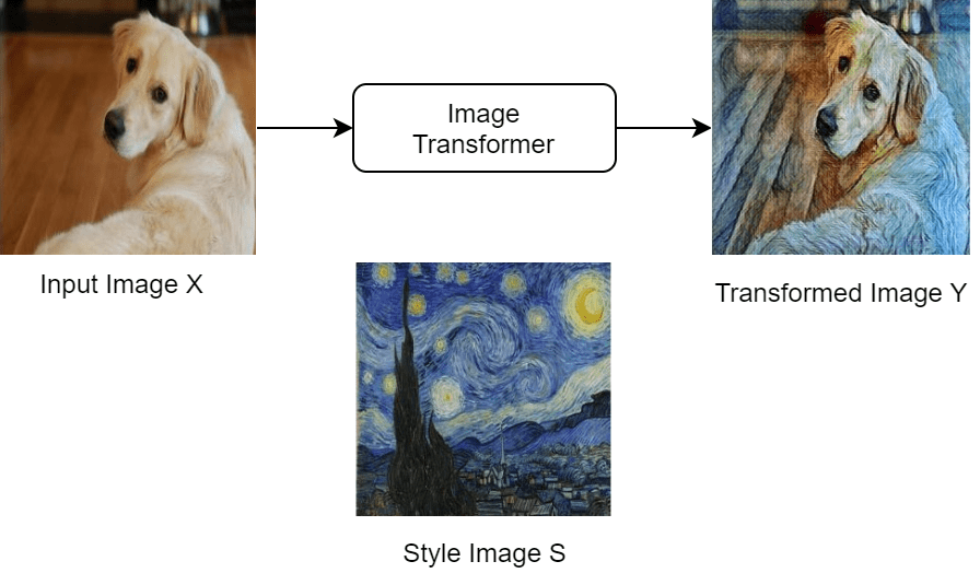
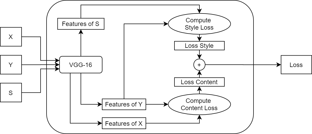
Find a high-level diagram of the training algorithm below. This uses three images to calculate the loss: the input image X, the transformed image Y and the style image S.

Note that the loss function uses the pretrained network VGG-16 to extract features from the images. You can find its implementation and mathematical definition in the Style Transfer Loss section of this example.
Load Training Data
Download and extract the COCO 2014 train images and captions from https://cocodataset.org/#download by clicking the "2014 Train images". Save the data in the folder specified by imageFolder. Extract the images into imageFolder. The COCO 2014 was collected by the Coco Consortium.
Create directories to store the COCO data set.
imageFolder = fullfile(tempdir,"coco");
if ~exist(imageFolder,"dir")
    mkdir(imageFolder);
end
Create an image datastore containing the COCO images.
imds = imageDatastore(imageFolder,IncludeSubfolders=true);
Training can take a long time to run. If you want to decrease the training time at the cost of accuracy of the resulting network, then select a subset of the image datastore by setting fraction to a smaller value.
fraction = 1;
numObservations = numel(imds.Files);
imds = subset(imds,1:floor(numObservations*fraction));
To resize the images and convert them all to RGB, create an augmented image datastore.
augimds = augmentedImageDatastore([256 256],imds,ColorPreprocessing="gray2rgb");Read the style image.
styleImage = imread("starryNight.jpg");
styleImage = imresize(styleImage,[256 256]);
Display the chosen style image.
figure
imshow(styleImage)
title("Style Image")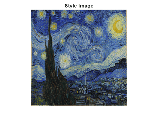
Define Image Transformer Network
Create a dlnetwork object.
netTransform = dlnetwork;
Specify the layers of the image transformer network and add them to the network. This is an image-to-image network. The network consists of 3 parts:
The first part of the network takes as input an RGB image of size [256x256x3] and downsamples it to a feature map of size [64x64x128].
The second part of the network consists of five identical residual blocks defined in the supporting function
residualBlock.The third and final part of the network upsamples the feature map to the original size of the image and returns the transformed image. This last part uses the
upsampleLayer, which is a custom layer attached to this example as a supporting file.
layers = [

    % First part.
    imageInputLayer([256 256 3],Normalization="none")

    convolution2dLayer([9 9],32,Padding="same")
    groupNormalizationLayer("channel-wise")
    reluLayer

    convolution2dLayer([3 3],64,Stride=2,Padding="same")
    groupNormalizationLayer("channel-wise")
    reluLayer

    convolution2dLayer([3 3],128,Stride=2,Padding="same")
    groupNormalizationLayer("channel-wise")
    reluLayer(Name="relu_3")

    % Second part.
    residualBlock("1")
    residualBlock("2")
    residualBlock("3")
    residualBlock("4")
    residualBlock("5")

    % Third part.
    upsampleLayer
    convolution2dLayer([3 3],64,Padding="same")
    groupNormalizationLayer("channel-wise")
    reluLayer

    upsampleLayer
    convolution2dLayer([3 3],32,Padding="same")
    groupNormalizationLayer("channel-wise")
    reluLayer

    convolution2dLayer(9,3,Padding="same")];

netTransform = addLayers(netTransform,layers);
Add missing connections in residual blocks.
netTransform = connectLayers(netTransform,"relu_3","add_1/in2");
netTransform = connectLayers(netTransform,"add_1","add_2/in2");
netTransform = connectLayers(netTransform,"add_2","add_3/in2");
netTransform = connectLayers(netTransform,"add_3","add_4/in2");
netTransform = connectLayers(netTransform,"add_4","add_5/in2");
Initialize the network.
netTransform = initialize(netTransform);
Visualize the image transformer network in a plot.
figure
plot(netTransform)
title("Transform Network")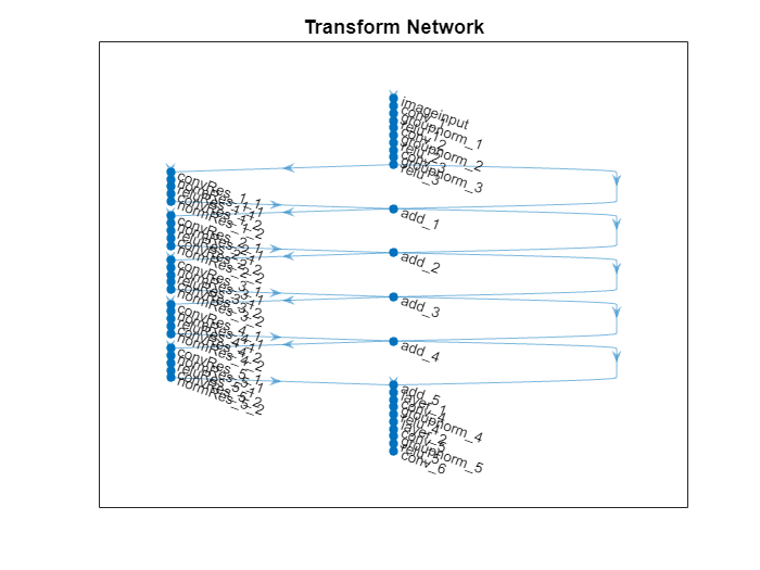
Style Loss Network
This example uses a pretrained VGG-16 deep neural network to extract the features of the content and style images at different layers. These multilayer features are used to compute respective content and style losses.
To get a pretrained VGG-16 network, use the imagePretrainedNetwork function. If you do not have the required support packages installed, then the software provides a download link.
netLoss = imagePretrainedNetwork("vgg16");Define Model Loss Function
Create the function modelLoss, listed in the Model Loss Function section of the example. This function takes as input the loss network, the image transformer network, a mini-batch of input images, an array containing the Gram matrices of the style image, the weight associated with the content loss and the weight associated with the style loss. The function returns the total loss, the loss associated with the content and the loss associated with the style, the gradients of the total loss with respect to the learnable parameters of the image transformer, the state of the image transformer network, and the transformed images.
Specify Training Options
Train with a mini-batch size of 16 for 2 epochs.
numEpochs = 2;
miniBatchSize = 16;
Set the read size of the augmented image datastore to the mini-batch size.
augimds.MiniBatchSize = miniBatchSize;
Specify the options for Adam optimization. Specify a learn rate of 0.001 with a gradient decay factor of 0.01, and a squared gradient decay factor of 0.999.
learnRate = 0.001;
gradientDecayFactor = 0.9;
squaredGradientDecayFactor = 0.999;
Specify the weight given to the style loss and the one given to the content loss in the calculation of the total loss.
Note that, in order to find a good balance between content and style loss, you might need to experiment with different combinations of weights.
weightContent = 1e-4;
weightStyle = 3e-8;
Choose the plot frequency of the training progress. This specifies how many iterations there are between each plot update.
plotFrequency = 100;
Train Model
In order to be able to compute the loss during training, calculate the Gram matrices for the style image.
Convert the style image to dlarray.
S = dlarray(single(styleImage),"SSC");In order to calculate the Gram matrix, feed the style image to the VGG-16 network and extract the activations at four different layers.
[SActivations1,SActivations2,SActivations3,SActivations4] = forward(netLoss,S, ...
    Outputs=["relu1_2" "relu2_2" "relu3_3" "relu4_3"]);
Calculate the Gram matrix for each set of activations using the supporting function createGramMatrix.
SGram{1} = createGramMatrix(SActivations1);
SGram{2} = createGramMatrix(SActivations2);
SGram{3} = createGramMatrix(SActivations3);
SGram{4} = createGramMatrix(SActivations4);
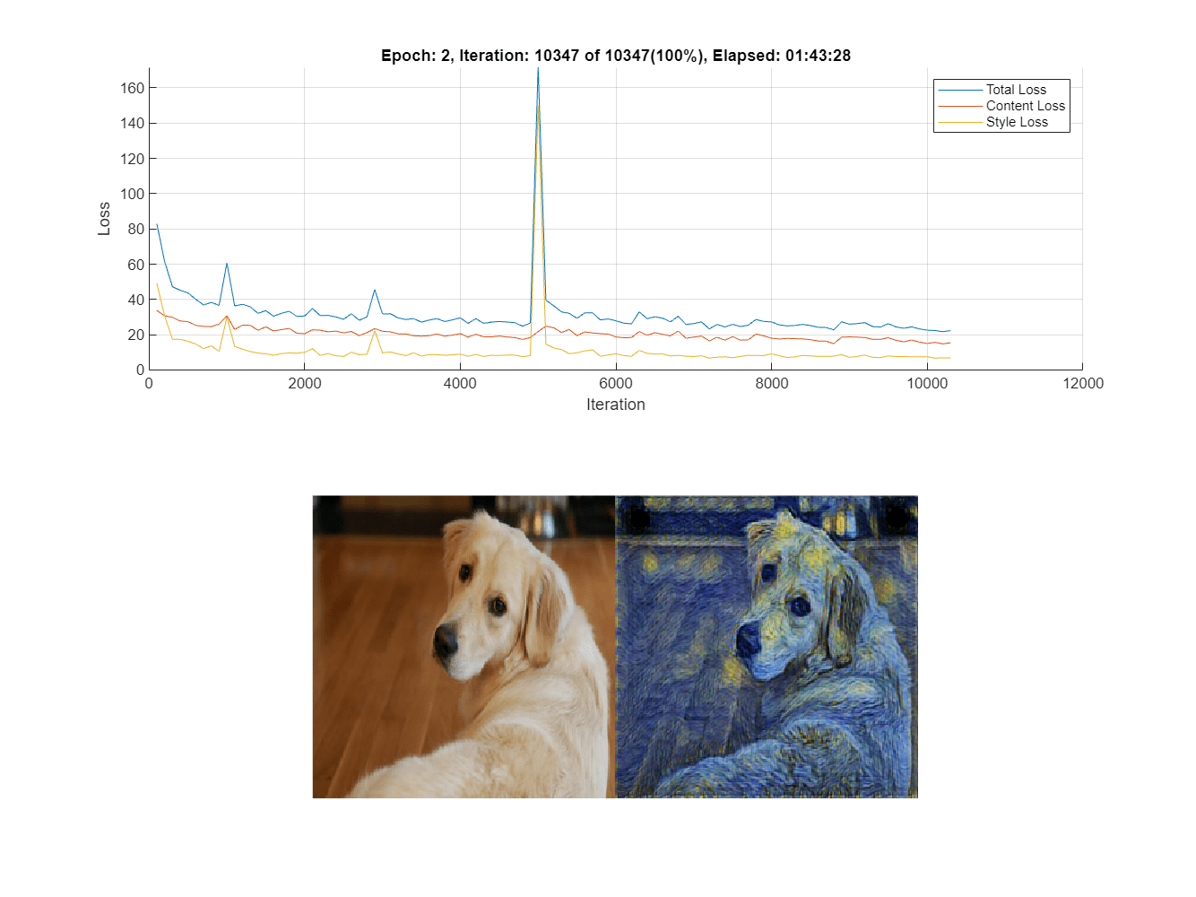
The training plots consists of two figures:
A figure showing a plot of the losses during training
A figure containing an input and an output image of the image transformer network
Initialize the training plots. You can check the details of the initialization in the supporting function initializeFigures. This function returns: the axis ax1 where you plot the loss, the axis ax2 where you plot the validation images, the animated line lineLossContent which contains the content loss, the animated line lineLossStyle which contains the style loss and the animated line lineLossTotal which contains the total loss.
[ax1,ax2,lineLossContent,lineLossStyle,lineLossTotal] = initializeStyleTransferPlots;
Initialize the average gradient and average squared gradient hyperparameters for the Adam optimizer.
averageGrad = [];
averageSqGrad = [];
Calculate total number of training iterations.
numIterations = floor(augimds.NumObservations*numEpochs/miniBatchSize);
Initialize iteration number and timer before training.
iteration = 0;
start = tic;
Train the model. Train on a GPU if one is available. Using a GPU requires Parallel Computing Toolbox™ and a supported GPU device. For information on supported devices, see GPU Computing Requirements (Parallel Computing Toolbox). This could take a long time to run.
% Loop over epochs.
for i = 1:numEpochs

    % Reset and shuffle datastore.
    reset(augimds);
    augimds = shuffle(augimds);

    % Loop over mini-batches.
    while hasdata(augimds)
        iteration = iteration + 1;

        % Read mini-batch of data.
        data = read(augimds);

        % Ignore last partial mini-batch of epoch.
        if size(data,1) < miniBatchSize
            continue
        end

        % Extract the images from data store into a cell array.
        images = data{:,1};

        % Concatenate the images along the 4th dimension.
        X = cat(4,images{:});
        X = single(X);

        % Convert mini-batch of data to dlarray and specify the dimension labels
        % "SSCB" (spatial, spatial, channel, batch).
        X = dlarray(X,"SSCB");

        % If training on a GPU, then convert data to gpuArray.
        if canUseGPU
            X = gpuArray(X);
        end

        % Evaluate the model loss, gradients, and the network state using
        % dlfeval and the modelLoss function listed at the end of the
        % example.
        [loss,lossContent,lossStyle,gradients,state,Y] = dlfeval(@modelLoss, ...
            netLoss,netTransform,X,SGram,weightContent,weightStyle);

        netTransform.State = state;

        % Update the network parameters.
        [netTransform,averageGrad,averageSqGrad] = ...
            adamupdate(netTransform,gradients,averageGrad,averageSqGrad,iteration,...
            learnRate, gradientDecayFactor,squaredGradientDecayFactor);

        % Every plotFrequency iterations, plot the training progress.
        if mod(iteration,plotFrequency) == 0
            addpoints(lineLossTotal,iteration,double(loss))
            addpoints(lineLossContent,iteration,double(lossContent))
            addpoints(lineLossStyle,iteration,double(lossStyle))

            % Use the first image of the mini-batch as a validation image.
            XV = X(:,:,:,1);
            % Use the transformed validation image computed previously.
            YV = Y(:,:,:,1);

            % To use the function imshow, convert to uint8.
            validationImage = uint8(gather(extractdata(XV)));
            transformedValidationImage = uint8(gather(extractdata(YV)));

            % Plot the input image and the output image and increase size
            imshow(imtile({validationImage,transformedValidationImage}),Parent=ax2);
        end

        % Display time elapsed since start of training and training completion percentage.
        D = duration(0,0,toc(start),Format="hh:mm:ss");
        completionPercentage = round(iteration/numIterations*100,2);
        title(ax1,"Epoch: " + i + ", Iteration: " + iteration +" of "+ numIterations + "(" + completionPercentage + "%)" +", Elapsed: " + string(D))
        drawnow

    end

end
Stylize an Image
Once training has finished, you can use the image transformer on any image of your choice.
Load the image you would like to transform.
imFilename = "peppers.png";
im = imread(imFilename);
Resize the input image to the input dimensions of the image transformer.
im = imresize(im,[256,256]);
Convert it to dlarray.
X = dlarray(single(im),"SSCB");To use the GPU convert to gpuArray if one is available.
if canUseGPU
    X = gpuArray(X);
end
To apply the style to the image, forward pass it to the image transformer using the function predict.
Y = predict(netTransform,X);
Rescale the image into the range [0 255]. First, use the function tanh to rescale Y to the range [-1 1]. Then, shift and scale the output to rescale into the [0 255] range.
Y = 255*(tanh(Y)+1)/2;
Prepare Y for plotting. Use the function extractdata to extract the data from dlarray. Use the function gather to transfer Y from the GPU to the local workspace.
Y = uint8(gather(extractdata(Y)));
Show the input image (left) next to the stylized image (right).
figure
m = imtile({im,Y});
imshow(m)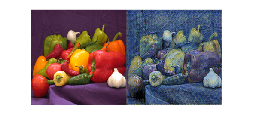
Model Loss Function
The function modelLoss takes as input the loss network netLoss, the image transformer network netTransform, a mini-batch of input images X, an array containing the Gram matrices of the style image SGram, the weight associated with the content loss contentWeight and the weight associated with the style loss styleWeight. The function returns the total loss, the loss associated with the content lossContent and the loss associated with the style lossStyle, the gradients of the total loss with respect to the learnable parameters of the image transformer gradients, the state of the image transformer network state, and the transformed images Y.
function [loss,lossContent,lossStyle,gradients,state,Y] = ...
    modelLoss(netLoss,netTransform,X,SGram,contentWeight,styleWeight)

[Y,state] = forward(netTransform,X);

Y = 255*(tanh(Y)+1)/2;

[loss,lossContent,lossStyle] = styleTransferLoss(netLoss,Y,X,SGram,contentWeight,styleWeight);

gradients = dlgradient(loss,netTransform.Learnables);

end
Style Transfer Loss
The function styleTransferLoss takes as input the loss network netLoss, a mini-batch of input images X, a mini-batch of transformed images Y, an array containing the Gram matrices of the style image SGram, the weights associated with the content and style contentWeight and styleWeight, respectively. It returns the total loss loss and the individual components: the content loss lossContent and the style loss lossStyle.
The content loss is a measure of how much difference in spatial structure there is between the input image X and the output images Y.
On the other hand, the style loss tells you how much difference in the stylistic appearance there is between the style image S and the output image Y.
The graph below explains the algorithm that styleTransferLoss implements to calculate the total loss.
First, the function passes the input images X, the transformed images Y and the style image S to the pretrained network VGG-16. This pretrained network extracts several features from these images. The algorithm then calculates the content loss by using the spatial features of the input image X and of the output image Y. Moreover, it calculates the style loss by using the stylistic features of the output image Y and of the style image S. Finally, it obtains the total loss by adding the content and style losses.
Content Loss
For each image in the mini-batch, the content loss function compares the features of the original image and of the transformed image output by the layer relu3_3. In particular, it calculates the mean squared error between the activations and returns the average loss for the mini-batch:
where contains the input images, contains the transformed images, is the mini-batch size, and represents the activations extracted at layer relu3_3.
Style Loss
To calculate the style loss, for each single image in the mini-batch:
Extract the activations at the layers
relu1_2,relu2_2,relu3_3andrelu4_3.For each of the four activations compute the Gram matrix .
Calculate the squared difference between the corresponding Gram matrices.
Add up the four outputs for each layer from the previous step.
To obtain the style loss for the whole mini-batch, compute the average of the style loss for each image in the mini-batch:
where is the index of the layer, and is the Gram Matrix.
Total Loss
function [loss,lossContent,lossStyle] = styleTransferLoss(netLoss,Y,X, ...
    SGram,weightContent,weightStyle)

% Extract activations.
YActivations = cell(1,4);
[YActivations{1},YActivations{2},YActivations{3},YActivations{4}] = ...
    forward(netLoss,Y,Outputs=["relu1_2" "relu2_2" "relu3_3" "relu4_3"]);

XActivations = forward(netLoss,X,Outputs="relu3_3");

% Calculate the mean squared error between activations.
lossContent = mean((YActivations{3} - XActivations).^2,"all");

% Add up the losses for all the four activations.
lossStyle = 0;
for j = 1:4
    G = createGramMatrix(YActivations{j});
    lossStyle = lossStyle + sum((G - SGram{j}).^2,"all");
end

% Average the loss over the mini-batch.
miniBatchSize = size(X,4);
lossStyle = lossStyle/miniBatchSize;

% Apply weights.
lossContent = weightContent * lossContent;
lossStyle = weightStyle * lossStyle;

% Calculate the total loss.
loss = lossContent + lossStyle;

end
Residual Block
The residualBlock function returns an array of six layers. It consists of convolution layers, instance normalization layers, a ReLu layer and an addition layer. Note that groupNormalizationLayer('channel-wise') is simply an instance normalization layer.
function layers = residualBlock(name)

layers = [
    convolution2dLayer([3 3], 128,Padding="same",Name="convRes_"+name+"_1")
    groupNormalizationLayer("channel-wise",Name="normRes_"+name+"_1")
    reluLayer(Name="reluRes_"+name+"_1")
    convolution2dLayer([3 3],128,Padding="same",Name="convRes_"+name+"_2")
    groupNormalizationLayer("channel-wise",Name="normRes_"+name+"_2")
    additionLayer(2,Name="add_"+name)];

end
Gram Matrix
The function createGramMatrix takes as an input the activations of a single layer and returns a stylistic representation for each image in a mini-batch. The input is a feature map of size [H, W, C, N], where H is the height, W is the width, C is the number of channels and N is the mini-batch size. The function outputs an array G of size [C,C,N]. Each subarray G(:,:,k) is the Gram matrix corresponding to the image in the mini-batch. Each entry of the Gram matrix represents the correlation between channels and , because each entry in channel multiplies the entry in the corresponding position in channel :
where are the activations for the image in the mini-batch.
The Gram matrix contains information about which features activate together but has no information about where the features occur in the image. This is because the summation over height and width loses the information about the spatial structure. The loss function uses this matrix as a stylistic representation of the image.
function G = createGramMatrix(activations)

[h,w,numChannels] = size(activations,1:3);

features = reshape(activations,h*w,numChannels,[]);
featuresT = permute(features,[2 1 3]);

G = dlmtimes(featuresT,features) / (h*w*numChannels);

end
References
Johnson, Justin, Alexandre Alahi, and Li Fei-Fei. "Perceptual losses for real-time style transfer and super-resolution." European conference on computer vision. Springer, Cham, 2016.
See Also
dlnetwork | forward | predict | dlarray | dlgradient | dlfeval | adamupdate
Topics
- Custom Loss Functions
- Custom Training Loops
- Custom Training Loop Model Loss Functions
- Train Generative Adversarial Network (GAN)
- Generate Images Using Diffusion
- Train Network Using Custom Training Loop
- Specify Training Options in Custom Training Loop
- List of Deep Learning Layers
- Deep Learning Tips and Tricks