Prepare Data for Battery State of Charge Estimation Using Deep Learning
This example shows how to prepare data for training a deep learning model to estimate the state of charge (SOC) of a battery. Preparing your data correctly is an important step in training a deep learning model.

SOC is the level of charge of an electric battery relative to its capacity, measured as a percentage. This example uses simulated battery state of charge data with three input features (temperature, voltage, and current) and one output feature (SOC). This example uses data generated using the Battery State of Charge Estimation Using Deep Learning example. You can use this data to train a deep learning network to predict the state of charge given the temperature, voltage, and current.

This example is step two in a series of examples that take you through a battery state of charge estimation workflow. You can run each step independently or work through the steps in order. This example follows the Define Requirements for Battery State of Charge Estimation example. For more information about the full workflow, see Battery State of Charge Estimation Using Deep Learning.
Generate Data
This examples uses data generated using a variant of the Simulink® model in the Battery State-of-Charge Estimation (Simscape Battery) example. This model simulates a battery charging and discharging over several hours.
The data has three variables: battery temperature, voltage, and current. The output is the state of charge.
The data is taken at four ambient temperatures: -10, 0, 10, and 25 degrees Celsius.
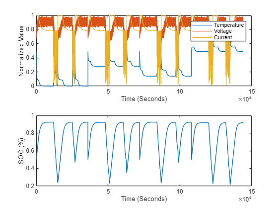
The battery charges for 9000 seconds and then discharges for 3000 seconds. This cycle repeats for 10 hours for each of the four ambient temperatures.
The initial state of charge is 0.5 and the battery charges to a state of charge of 0.9.
The model uses a Cycler block to simulate ideal charging and discharging.
Load Data
Load the training data. The data is attached to this example as supporting files. To access the data, open this example in MATLAB®. The data contains four MAT files, each corresponding to a different ambient temperature setting: -10, 0, 10, or 25 degrees Celsius. Each data set comprises a single sequence of experimental data captured as the battery powered an electric vehicle through a driving cycle at the specified temperatures.
rng("default")
datan10 = load(fullfile("BSOCTrainingData","BSOC_n10_degrees.mat"));
data0 = load(fullfile("BSOCTrainingData","BSOC_0_degrees.mat"));
data10 = load(fullfile("BSOCTrainingData","BSOC_10_degrees.mat"));
data25 = load(fullfile("BSOCTrainingData","BSOC_25_degrees.mat"));
View the data. Each temperature data variable contains a structure with the predictors (X) and the response (Y).
datan10
datan10 = struct with fields:
    X: [36001×3 double]
    Y: [0.5000 0.5002 0.5003 0.5005 0.5006 0.5008 0.5009 0.5011 0.5012 0.5014 0.5015 0.5017 0.5019 0.5020 0.5022 0.5023 0.5025 0.5026 0.5028 0.5029 0.5031 0.5032 0.5034 0.5035 0.5037 0.5039 0.5040 0.5042 0.5043 0.5045 0.5046 0.5048 … ] (1×36001 double)
Combine the four temperatures into a single observation.
X = [datan10.X; data0.X; data10.X; data25.X];
Y = [datan10.Y, data0.Y, data10.Y, data25.Y]';

data = struct;
data.X = X;
data.Y = Y;
When you train neural networks, data normalization is a best practice. Normalization helps stabilize and speed up network training using gradient descent. If your data is poorly scaled, then the deep learning training loss can become NaN and the network parameters can diverge during training. Common ways of normalizing data include rescaling the data so that its range becomes [0,1] or so that it has a mean of zero and standard deviation of one. For this example, rescale the predictors so that they are in the range [0,1]. You do not need to scale the responses (SOC) as these values are already between 0 and 1.
maxX = max(data.X);
minX = min(data.X);
data.X = rescale(data.X,InputMin=minX,InputMax=maxX);
Save the maximum and minimum training statistics. When you use this model for prediction, normalize the inputs using the training statistics.
save("trainingMaxMinStats","minX","maxX")
Visualize the data.
figure
tiledlayout(2,1)
nexttile
plot(data.X)
legend(["Temperature" "Voltage" "Current"])
xlabel("Time (Seconds)")
ylabel("Normalized Value")
nexttile
plot(data.Y)
xlabel("Time (Seconds)")
ylabel("SOC (%)")

Prepare Data
Prepare the data for training an LSTM deep learning model. Define the preprocessing function, chunkData, to split the data into chunks. Any remaining data that is less than a batch is discarded.
function [X,Y] = chunkData(data,chunkSize)

% Calculate number of samples and observations.
numSamples = length(data.Y);
numObservations = floor(numSamples/chunkSize);

X = cell(1,numObservations);
Y = cell(1,numObservations);

% Split the data.
for i = 1:numObservations
    idxStart = 1+(i-1)*chunkSize;
    idxEnd = i*chunkSize;
    X{i} = data.X(idxStart:idxEnd,:);
    Y{i} = data.Y(idxStart:idxEnd);
end
end
Preprocess the data using the preprocessing function. Split the data into chunks, each with 500 time steps.
chunkSize = 500;
[XData,YData] = chunkData(data,chunkSize);

numObservations = numel(YData)
numObservations =
288
Split the data into training and validation sets. Use 70% of the data for training and 30% for validation. Validation data is important for evaluating the performance of a model on unseen data during the training process. Validation helps to avoid overfitting and makes sure that the model generalizes well to new, unseen data.
numObservationsTrain = floor(0.7*numObservations)
numObservationsTrain =
201
numObservationsValidation = numObservations - numObservationsTrain
numObservationsValidation =
87
idx = randperm(numObservations);
idxTrain = idx(1:numObservationsTrain);
idxValidation = idx(numObservationsTrain+1:end);

XTrain = XData(idxTrain);
YTrain = YData(idxTrain);

XVal = XData(idxValidation);
YVal = YData(idxValidation);
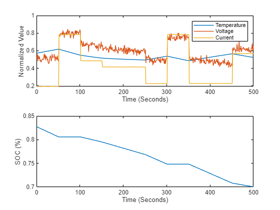
Visualize one of the observations.
idx = 1;

figure
tiledlayout(2,1)
nexttile
plot(XTrain{idx})
legend(["Temperature" "Voltage" "Current"])
xlabel("Time (Seconds)")
ylabel("Normalized Value")
nexttile
plot(YTrain{idx})
xlabel("Time (Seconds)")
ylabel("SOC (%)")
The data is now ready to use for deep learning model training. To train the model, see Train Deep Learning Network for Battery State of Charge Estimation. You can also open the next example using the openExample function.
openExample("deeplearning_shared/TrainModelForBatteryStateOfChargeEstimationExample")
Optionally, if you have Requirements Toolbox™, then in the next section, you can link and test data coverage requirements.
Link Data Requirements Using Requirements Toolbox
This section links the data to the requirements and requires Requirements Toolbox™ and MATLAB Test™. This section does not show how to create or link requirements, only how to implement and verify the links. For more information about defining these requirements, see Define Requirements for Battery State of Charge Estimation. For general information about how to create and manage requirements, see Use Requirements to Develop and Verify MATLAB Functions (Requirements Toolbox).
Linking data requirements is important for data traceability. You can use data requirements to check:
Quality — Ensure that your data is suitable for the task and is of sufficient quality.
Coverage — Ensure that your data has sufficient coverage for the task.
Reproducibility — Ensure that you can trace the data and reproduce the data collection and preparation.
Check for a Requirements Toolbox™ license.
if ~license("test","simulink_requirements")
    disp("This part of the example requires Requirements Toolbox.");
    return
end
In this example, focus on the data coverage requirement. The recorded SOC is dependent on the ambient temperature at which the data was taken. To ensure the prediction model generalizes well, data from a range of temperatures is necessary. In this example, the data must be for SOC taken at four temperatures: -10, 0, 10, and 25 degrees Celsius.
Open the data requirements. To add columns that indicate the implementation and verification status of the requirements, click Columns ![]() and then select Implementation Status and Verification Status. If you see a yellow banner, then click Analyze now. You can see each of the requirements and their implementation status and verification status. The verified status for each requirement is yellow, indicating that the status is unknown. The status turns to red if the requirement fails or green if the requirement passes.
and then select Implementation Status and Verification Status. If you see a yellow banner, then click Analyze now. You can see each of the requirements and their implementation status and verification status. The verified status for each requirement is yellow, indicating that the status is unknown. The status turns to red if the requirement fails or green if the requirement passes.
open("testTemperatureDataRequirements.m")
slreq.open("BatterySOCReqData.slreqx");

Select one of the data requirements. Each data requirement is implemented by TempJustification and verified by testTemperatureCoverage test. In the next sections, learn how to implement and verify each requirement.

Implement Requirements
In Requirements Editor, select the temperature justification. The description outlines that this requirement uses dataTraceTable to confirm the implementation status. The next steps show how to create dataTraceTable such that you can justify the implementation and then verify that the requirement is met.

Load the data requirements into a variable.
reqSet = slreq.load("BatterySOCReqData.slreqx");Get the functional requirement items.
dataReqs = find(reqSet,"Type","Requirement","Type","Functional");
Generate a table linking information about the data to each of the data requirements. The table contains:
Requirement ID
Size and format of the predictors
Size and format of the responses
Data for each temperature
Temperature value
dataTraceMatrix = cell(length(dataReqs),4);
temp = [-10 0 10 25];
for ii = 1:length(dataReqs)

    % Get requirement ID.
    dataTraceMatrix{ii,1} = dataReqs(ii).Id;

    data = load("BSOCTrainingData\" + dataReqs(ii).Id +".mat");

    % Specify number of observations.
    dataTraceMatrix{ii,2} = size(data.X);
    dataTraceMatrix{ii,3} = numel(data.Y);

    % Specify data format.
    dataTraceMatrix{ii,4} = "TC";
    dataTraceMatrix{ii,5} = "TC";

    dataTraceMatrix{ii,6} = data;
    dataTraceMatrix{ii,7} = temp(ii);
end
Convert the data traceability matrix to a table and display the result. The data traceability table covers the implementation of the data requirements.
dataTraceTable = cell2table(dataTraceMatrix, ...
    VariableNames=["Data Requirement ID","Predictors Size", ...
    "Response Size", "Predictors Format","Response Format", ...
    "Data", "Temperature"]);
View the table.
disp(dataTraceTable)
    Data Requirement ID     Predictors Size    Response Size    Predictors Format    Response Format       Data       Temperature
    ____________________    _______________    _____________    _________________    _______________    __________    ___________

    {'BSOC_n10_degrees'}    36001        3         36001              "TC"                "TC"          1×1 struct        -10
    {'BSOC_0_degrees'  }    36001        3         36001              "TC"                "TC"          1×1 struct          0
    {'BSOC_10_degrees' }    36001        3         36001              "TC"                "TC"          1×1 struct         10
    {'BSOC_25_degrees' }    36001        3         36001              "TC"                "TC"          1×1 struct         25
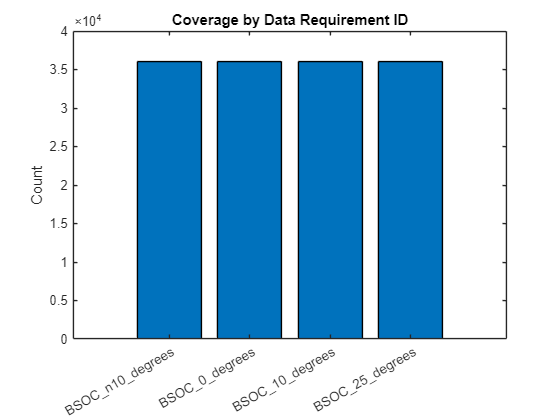
Create a bar chart where the -axis represents the requirements IDs and the -axis provides the total length of the data that matches that requirement. You can see that the data requirement is met for each temperature.
figure
bar(dataTraceTable.("Response Size"));
xticklabels(dataTraceTable.("Data Requirement ID"))
title("Coverage by Data Requirement ID")
ylabel("Count")

ax = gca;
ax.TickLabelInterpreter = "none";

Save the traceability matrix table with the name dataTraceTable. You will use this table to verify the data requirements.
save("dataTraceTable","dataTraceTable");
Verify Requirements
The next step is to formally verify the requirements. To verify requirements, create tests to check the data coverage. You can find the data tests in the testTemperatureDataRequirements file, attached to this example as a supporting file. These tests take as input the generated dataTraceTable and check that each temperatures has at least a single data point.
        function testTemperatureCoverage(testCase,tempArray)

            % Check the data trace table has been generated.
            assertThat(testCase,"dataTraceTable.mat", matlab.unittest.constraints.IsFile, ...
                "Test failed. Unable to load dataTraceTable.mat. To load this table," + ...
                " run the Prepare Data for Battery State of Charge Estimation Using Deep Learning Example.");

            load("dataTraceTable.mat");

            % Access the data for the specified temperature.
            rowIdx = dataTraceTable.Temperature == tempArray;
            temperatureData = dataTraceTable(rowIdx,:);

            dataLength = temperatureData.("Response Size");

            % Check that there is at least one observation.
            verifyGreaterThan(testCase,dataLength,0);
        end
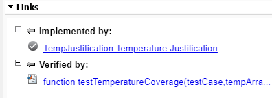
When you open the test file, you can see that the software highlights the test name. Highlighted tests are linked to requirements. To see which requirement the test links to, right click on the line and select Requirements.
![]()
In Requirements Editor, right-click on the requirements set BatterySOCReqData and click Run Tests. In the Run Tests dialog box, select the testTemperatureCoverage test and click Run Tests. Doing so runs all the tests linked to these requirements.

The tests check that each of the temperature requirements are met and the verification status turns to green (Passed).

Next step: Train Deep Learning Network for Battery State of Charge Estimation. You can also open the next example using the openExample function.
openExample("deeplearning_shared/TrainModelForBatteryStateOfChargeEstimationExample")
See Also
Requirements Editor (Requirements Toolbox)