Test Deep Learning Network for Battery State of Charge Estimation

Test Network

Calculate the difference between the predicted SOC and the target SOC for four different ambient temperatures. This example tests the model on data with the ambient temperatures -10 ("n10"), 0, 10, and 5 degrees Celsius.

temperature = ["n10" "0" "10" "25"];

For each temperature:

dataTrue = [];
YPred = [];
TestRMSE = [];

for i = 1:4

    % Load test data.
    filename = "BSOC_" + temperature(i) + "_degrees.mat";
    testFile = fullfile("BSOCTestingData",filename);
    dataTrue{i} = load(testFile);

    % Normalize data.
    load("BSOCTrainingMaxMinStats.mat")
    dataTrue{i}.X = rescale(dataTrue{i}.X,InputMin=minX,InputMax=maxX);

    % Generate predictions.
    YPred{i} = minibatchpredict(recurrentNet,dataTrue{i}.X);

    % Compute the residuals and RMSE.
    residuals = dataTrue{i}.Y - YPred{i}';
    TestRMSE(i) = sqrt(mean(residuals.^2));
end

Plot the residuals for each temperature.

figure
tiledlayout("flow")

for i = 1:4
    nexttile
    plot(residuals)
    title("Residuals (Temperature: " + temperature(i) + "°C)","RMSE: " + TestRMSE(i))
    xlabel("Time")
    ylabel("Residuals")
end

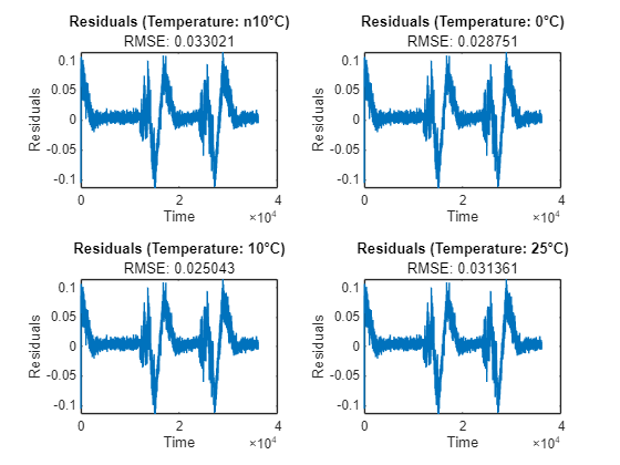
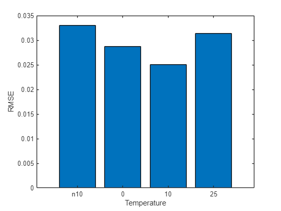
Compare the RMSE for each temperature.

figure
bar(temperature,TestRMSE)
xlabel("Temperature")
ylabel("RMSE")

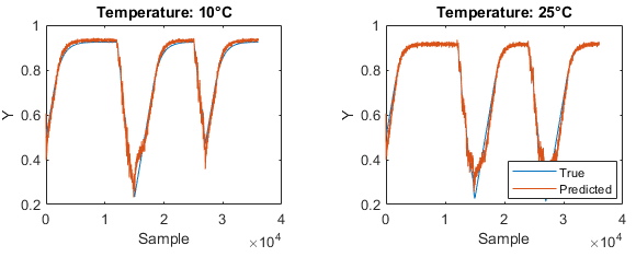
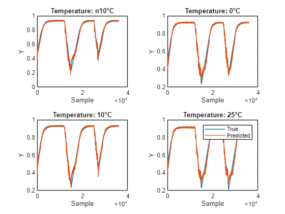
For each temperature, use test data to compare the SOC predicted by the network and the target SOC. Plot the predicted and the target SOC for each ambient temperature.

figure
tiledlayout("flow")
for i = 1:4
    nexttile
    plot(dataTrue{i}.Y);
    hold on
    plot(YPred{i})
    hold off
    xlabel("Sample")
    ylabel("Y")
    if i == 4
        legend(["True" "Predicted"])
    end
    title("Temperature: " + temperature(i) + "°C")
end

Verify Robustness to Out-of-Distribution Data

Out-of-distribution (OOD) data detection is the process of identifying inputs to a deep neural network that might yield unreliable predictions. OOD data refers to data that is different from the data used to train the model, for example, data collected in a different way, at a different time, under different conditions, or for a different task than the data on which the model was originally trained. You can use the Deep Learning Toolbox Verification Library support package to detect inputs that the network has not seen before.

Create OOD Data Discriminator

To detect OOD data, create a data discriminator. You can use the discriminator to classify inputs as either OOD or in-distribution (ID). To create an OOD data discriminator, use the networkDistributionDiscriminator function. To use the OOD functions, create a minibatchqueue object.

mbqTrain = minibatchqueue(...
    arrayDatastore(XTrain',IterationDimension=1,OutputType="same",ReadSize=numel(XTrain)), ...
    MiniBatchSize=32, ...
    MiniBatchFormat="TCB", ...
    MiniBatchFcn=@(X) cat(3,X{:}));

To create a data discriminator, you must have:

Use the networkDistributionDiscriminator function with the network and training data as input. Because the task is a regression task, set the method to "hbos". The discriminator is an object that you can use to detect OOD data.

discriminator = networkDistributionDiscriminator(recurrentNet,mbqTrain,[],"hbos", ...
    VerbosityLevel="off",TruePositiveGoal=0.95);

Create OOD Data

In this example, simulate OOD data by adding drift to the voltage variable. Adding drift simulates a sensor failing. Add noise to 40 observations.

numNoisyObs = 40;
oodXValNoisy = XVal;
randomIdx = randperm(numel(oodXValNoisy),numNoisyObs);
noiseIdx = randomIdx(1:40);

% Add drift to the second variable (voltage).
for ii = noiseIdx
    oodXValNoisy{ii} = oodXValNoisy{ii} + ([0; -0.0004; 0].*(1:500))';
end

View one of the noisy observations.

idx = 5;
figure
plot(XVal{noiseIdx(idx)}(:,2))
xlabel("Time")
ylabel("Voltage")
hold on
plot(oodXValNoisy{noiseIdx(idx)}(:,2))
hold off
legend(["Original","Noisy"])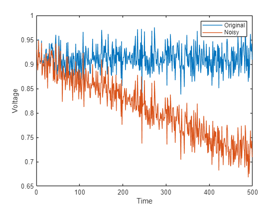

Convert the noisy data into a minibatchqueue object.

dsValNoisy = arrayDatastore(oodXValNoisy',IterationDimension=1,OutputType="same",ReadSize=numel(oodXValNoisy));
mbqValNoisy = minibatchqueue(dsValNoisy, ...
    MiniBatchSize=32, ...
    MiniBatchFormat="TCB", ...
    MiniBatchFcn=@(X) cat(3,X{:}));

Detect OOD Data

To detect OOD data, use the isInNetworkDistribution function. This function takes as input a discriminator and a set of data and returns an array where each element is 1 if the discriminator predicts that observation to be ID and 0 if OOD.

Use the discriminator with the noisy data.

OODClass = isInNetworkDistribution(discriminator,mbqValNoisy);

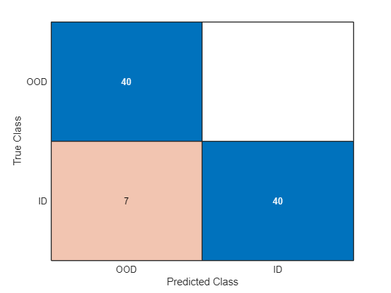
A working discriminator detects the non-noisy data as ID and the noisy data as OOD. Check the accuracy of the discriminator.

target = ones(numel(oodXValNoisy),1);
target(noiseIdx) = 0;

sum(OODClass == target)/numel(oodXValNoisy)

ans =

    0.9195

The discriminator achieves a high accuracy and is able to discriminate between the ID and OOD data. Plot the confusion matrix.

targetName = categorical(target,[0 1],["OOD" "ID"]); 
OODClassName = categorical(OODClass,[0 1],["OOD" "ID"]); 

confusionchart(targetName,OODClassName)

Now that the network is tested, you can integrate it into a Simulink model. To integrate the network into a Simulink model, see Integrate AI Model into Simulink for Battery State of Charge Estimation. You can also open the next example using the openExample function.

openExample("deeplearning_shared/AIModelSimulinkForBatteryStateOfChargeEstimationExample")

Optionally, if you have Requirements Toolbox™, then in the next section, you can link and test network inference requirements.

Link Network Inference Requirements Using Requirements Toolbox

This section links the network predictions to the requirements and requires Requirements Toolbox™ and MATLAB Test™. This section does not show how to create or link requirements, only how to implement and verify the links. For more information about defining these requirements, see Define Requirements for Battery State of Charge Estimation. For general information about how to create and manage requirements, see Use Requirements to Develop and Verify MATLAB Functions.

Linking network inference requirements is important for ensuring that your network achieves suitable performance, generalizes well, and is robust to out-of-distribution data.

Check for a Requirements Toolbox™ license.

if ~license("test","simulink_requirements")    
    disp("This part of the example requires Requirements Toolbox.");    
    return
end

Save the RMSE and OOD results. You will use these to test the network requirements.

save("RMSEResults","TestRMSE");
save("OODResults.mat", "OODClass", "target");

Open the network inference requirements. To add columns that indicate the implementation status and verification status of the requirements, click Columns and then select Implementation Status and Verification Status. If you see a yellow banner, then click Analyze now to view the implemented and verified status. You can see each of the requirements and their implementation status and verification status. The verification status for each requirement is yellow, indicating that the status is unknown. The status turns to red if the requirement fails or green if the requirement passes.

open("testNetworkInferenceRequirements.m")
slreq.open("BatterySOCReqNetInfe.slreqx");

Select one of the network requirements. Each requirement is implemented by NetworkInfeJustification and verified by a test.

Implement Requirements

By creating a network capable of achieving the required RMSE value, you have implemented the requirements. You can see this justification by selecting NetworkInputOutputJustification in the requirements editor.

Verify Requirements

The next step is to formally verify the requirements. To verify requirements, create tests to check the network performance. You can find the network inference tests in the testNetworkInferenceRequirements file, attached to this example as a supporting file. The file contains two tests:

        function testRMSEThresholdForEachTemperature(testCase)
            threshold = 0.05;
            verifyLessThan(testCase,testCase.RMSEValues,threshold);
        end

        function testOutOfDistribution(testCase)
            targetAccuracy = 0.9;

            achievedAccuracy = sum(testCase.OODClass == testCase.TrueClass )/numel(testCase.OODClass);

            verifyGreaterThanOrEqual(testCase,achievedAccuracy,targetAccuracy);
        end

When you open the test file, you can see that the software highlights the test names. Highlighted tests are linked to requirements. To see which requirement a test links to, right-click the line and select Requirements.

In Requirements Editor, right-click the requirements set BatterySOCReqNetInfe and click Run Tests. In the Run Tests dialog box, select the testRMSEThresholdForEachTemperature and testOutOfDistribution tests and click Run Tests. The tests check that each of the network requirements are met and the verification status turns to green (Passed).

Next step: Integrate AI Model into Simulink for Battery State of Charge Estimation. You can also open the next example using the openExample function.

openExample("deeplearning_shared/AIModelSimulinkForBatteryStateOfChargeEstimationExample")