训练具有多个输出的网络
此示例说明如何训练具有多个输出的深度学习网络,来预测手写数字的标签和旋转角度。
加载训练数据
加载数字数据。该数据包含数字的图像和数字标签,以及它们与垂直方向的旋转角度。
load DigitsDataTrain为图像、标签和角度创建一个 arrayDatastore 对象,然后使用 combine 函数创建一个包含所有训练数据的数据存储。
dsXTrain = arrayDatastore(XTrain,IterationDimension=4);
dsT1Train = arrayDatastore(labelsTrain);
dsT2Train = arrayDatastore(anglesTrain);

dsTrain = combine(dsXTrain,dsT1Train,dsT2Train);

classNames = categories(labelsTrain);
numClasses = numel(classNames);
numObservations = numel(labelsTrain);
查看训练数据中的一些图像。
idx = randperm(numObservations,64);
I = imtile(XTrain(:,:,:,idx));
figure
imshow(I)

定义深度学习模型
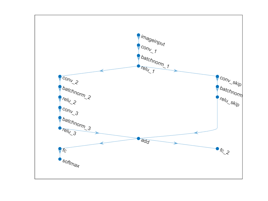
定义以下网络,用于预测标签和旋转角度。
具有 16 个 5×5 滤波器的 convolution-batchnorm-ReLU 模块。
每个模块具有 32 个 3×3 滤波器的两个 convolution-batchnorm-ReLU 模块。
围绕上述两个模块的跳过连接,包含一个具有 32 个 1×1 卷积的 convolution-batchnorm-ReLU 模块。
使用加法合并跳过连接。
对于分类输出,一个具有大小为 10(类数)的全连接运算和 softmax 运算的分支。
对于回归输出,一个具有大小为 1(响应数)的全连接运算的分支。
定义层的主要模块。
net = dlnetwork;

layers = [
    imageInputLayer([28 28 1],Normalization="none")

    convolution2dLayer(5,16,Padding="same")
    batchNormalizationLayer
    reluLayer(Name="relu_1")

    convolution2dLayer(3,32,Padding="same",Stride=2)
    batchNormalizationLayer
    reluLayer
    convolution2dLayer(3,32,Padding="same")
    batchNormalizationLayer
    reluLayer

    additionLayer(2,Name="add")

    fullyConnectedLayer(numClasses)
    softmaxLayer(Name="softmax")];

net = addLayers(net,layers);
添加跳过连接。
layers = [
    convolution2dLayer(1,32,Stride=2,Name="conv_skip")
    batchNormalizationLayer
    reluLayer(Name="relu_skip")];

net = addLayers(net,layers);
net = connectLayers(net,"relu_1","conv_skip");
net = connectLayers(net,"relu_skip","add/in2");
为回归添加全连接层。
layers = fullyConnectedLayer(1,Name="fc_2");
net = addLayers(net,layers);
net = connectLayers(net,"add","fc_2");
查看绘图中的层图。
figure
plot(net)
指定训练选项
指定训练选项。在选项中进行选择需要经验分析。要通过运行试验探索不同训练选项配置,您可以使用Experiment Manager。
options = trainingOptions("adam", ...
    Plots="training-progress", ...
    Verbose=false);
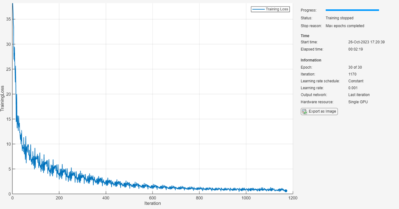
训练神经网络
使用 trainnet 函数训练神经网络。对于分类,请使用自定义损失函数,该函数是预测标签和目标标签的交叉熵损失加上预测角度和目标角度的均方误差损失的 0.1 倍。默认情况下,trainnet 函数使用 GPU(如果有)。使用 GPU 需要 Parallel Computing Toolbox™ 许可证和受支持的 GPU 设备。有关受支持设备的信息,请参阅GPU 计算要求 (Parallel Computing Toolbox)。否则,该函数使用 CPU。要指定执行环境,请使用 ExecutionEnvironment 训练选项。
将自定义损失函数定义为函数句柄。定义一个损失,该损失对应于预测标签和目标标签的交叉熵损失加上预测角度和目标角度的均方误差,按 0.1 因子进行缩放。
lossFcn = @(Y1,Y2,T1,T2) crossentropy(Y1,T1) + 0.1*mse(Y2,T2);
训练神经网络。
net = trainnet(dsTrain,net,lossFcn,options);
测试模型
加载数字数据。该数据包含数字的图像和数字标签,以及它们与垂直方向的旋转角度。
load DigitsDataTest使用 minibatchpredict 函数进行预测,并使用 scores2label 函数将分类分数转换为标签。默认情况下,minibatchpredict 函数使用 GPU(如果有)。使用 GPU 需要 Parallel Computing Toolbox™ 许可证和受支持的 GPU 设备。有关受支持设备的信息,请参阅GPU 计算要求 (Parallel Computing Toolbox)。否则,该函数使用 CPU。要手动选择执行环境,请使用 minibatchpredict 函数的 ExecutionEnvironment 参量。
[scores,Y2] = minibatchpredict(net,XTest);
Y1 = scores2label(scores,classNames);
计算标签的分类准确度。
accuracy = mean(Y1 == labelsTest)
accuracy = 0.9732
计算预测角度和目标角度之间的均方根误差。
err = rmse(Y2,anglesTest)
err = single
    6.9265
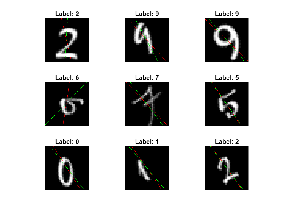
查看其中一些图像及其预测值。用红色显示预测角度,用绿色显示正确标签。
idx = randperm(size(XTest,4),9);
figure
for i = 1:9
    subplot(3,3,i)
    I = XTest(:,:,:,idx(i));
    imshow(I)
    hold on

    sz = size(I,1);
    offset = sz/2;

    theta = Y2(idx(i));
    plot(offset*[1-tand(theta) 1+tand(theta)],[sz 0],"r--")

    thetaTest = anglesTest(idx(i));
    plot(offset*[1-tand(thetaTest) 1+tand(thetaTest)],[sz 0],"g--")

    hold off
    label = Y1(idx(i));
    title("Label: " + string(label))
end
另请参阅
trainnet | trainingOptions | dlnetwork | batchNormalizationLayer | convolution2dLayer | reluLayer | fullyConnectedLayer | softmaxLayer | minibatchqueue