Train Transolver Neural Network for 3-D Electrostatic Field Prediction

R2026b

Since R2026b

This example uses:

This example shows how to train a Transolver neural network to predict electric potential fields for a 3-D electrostatics problem.

A Transolver neural network is a type of transformer neural network that learns to approximate solutions to partial differential equations (PDEs) by partitioning input tokens into physics-aware slices. Transolver neural networks are well suited for problems involving complex geometries and irregular meshes, such as computational fluid dynamics and electromagnetic simulations. You can use Transolver neural networks to replace computationally expensive numerical solvers with fast neural network inference, enabling rapid design exploration. Transolver neural networks can generate predictions orders of magnitude faster than full numerical simulations, particularly for iterative design workflows that require evaluating many geometry variations.

This example trains a Transolver neural network that predicts electric potential fields for 3-D electrostatic geometries. It prepares simulation data, defines and trains the neural network using a custom loss function, and evaluates predictions on test data. You can use the trained model to predict the electric potential for new bushing insulator designs without running a full simulation.

This diagram illustrates the workflow of using a Transolver neural network for electrostatic field prediction.

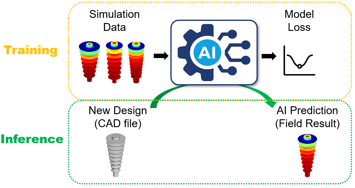
Training a Transolver neural network can take a long time. This example skips the training step and loads a pretrained neural network. To train the neural network in this example, set the doTrain variable to true.

doDataGeneration = false;
doTrain = false;

Load Data

Generate electrostatic simulation data using the generateElectrostaticSimulationData function. The function creates parameterized transformer bushing insulator geometries using Latin Hypercube Sampling, solves the 3-D electrostatic PDE for each geometry using Partial Differential Equation Toolbox, and returns a structure containing the mesh coordinates, material properties, electric potential, and electric field at each node.

The example generates the data and saves it for subsequent runs. To generate the data again, set the doDataGeneration variable to 1 (true). If the data file does not exist, then the example generates the data again and saves it.

dataFolder = fullfile(pwd,"data");
filenameData = fullfile(dataFolder,"electrostaticSimulationData.mat");

if doDataGeneration || ~exist(filenameData,"file")
    data = generateElectrostaticSimulationData;

    if ~exist(dataFolder,"dir")
        mkdir(dataFolder)
    end
    
    save(filenameData,"data")
else
    load electrostaticSimulationData
end

Prepare Data for Training

The training function requires predictors as numFeatures-by-numNodes numeric arrays and targets as 1-by-numNodes numeric arrays, where numFeatures is the number of input features (spatial coordinates and material properties) and numNodes is the number of mesh nodes.

Loop over the simulation results and extract the node coordinates and material properties as inputs and the electric potential as targets, subsampling to reduce computational cost.

stride = 10;

inputs = cell(numel(data),1);
targets = cell(numel(data),1);

for i = 1:numel(data)
    input = cat(1, ...
        data(i).Coord,...
        data(i).Epsilon');

    target = data(i).Potential';

    inputs{i} = input(:,1:stride:end);
    targets{i} = target(:,1:stride:end);
end

Split the data into training, validation, and test partitions using the trainingPartitions function, which is attached to this example as a supporting file. To access this function, open the example as a live script. Use 80% of the data for training, 10% for validation, and the remaining 10% for testing.

[idxTrain,idxVal,idxTest] = trainingPartitions(numel(inputs),[0.8 0.1 0.1]);

inputsTrain = inputs(idxTrain);
inputsVal = inputs(idxVal);
inputsTest = inputs(idxTest);
targetsTrain = targets(idxTrain);
targetsVal = targets(idxVal);
targetsTest = targets(idxTest);

Preprocess Data

To improve training, normalize the data, pad it to uniform length, set up random rotations and reflections for augmentation, and combine predictors and targets into datastores.

Define preprocessing functions for the input features and target potential values. For this example, preprocessing consists of normalization. If your workflow requires additional preprocessing steps, such as feature engineering or outlier removal, then include them in these functions to ensure consistent preprocessing between training and inference.

function U = preprocessElectrostaticInput(U, offset, scaleFactor)
    U = (U - offset) ./ scaleFactor;
end

function V = preprocessElectrostaticPotential(V, offset, scaleFactor)
    V = (V - offset) ./ scaleFactor;
end

Normalize the inputs and targets to the range [-1, 1]. For the spatial coordinates, use a single uniform scale factor across all three dimensions to preserve the aspect ratio of the geometry. The relative permittivity feature takes only two values (1 for air, 5 for the bushing insulator), so after normalization it acts as a categorical indicator: approximately -1 for air nodes and +1 for bushing nodes.

coordIdx = 1:3;

[rowMin, rowMax] = bounds([inputsTrain{:}], 2);

inputOffset = 0.5 * (rowMin + rowMax);
inputScale  = 0.5 * (rowMax - rowMin);

inputOffset(coordIdx) = 0;
s = max(inputScale(coordIdx));
inputScale(coordIdx) = s;

[rowMin, rowMax] = bounds([targetsTrain{:}], 2);

outputOffset = 0.5 * (rowMin + rowMax);
outputScale  = 0.5 * (rowMax - rowMin);

normalizedInputsTrain = cell(size(inputsTrain));
normalizedTargetsTrain = cell(size(targetsTrain));
for i = 1:numel(inputsTrain)
    normalizedInputsTrain{i} = preprocessElectrostaticInput(inputsTrain{i}, inputOffset, inputScale);
    normalizedTargetsTrain{i} = preprocessElectrostaticPotential(targetsTrain{i}, outputOffset, outputScale);
end

normalizedInputsVal = cell(size(inputsVal));
normalizedTargetsVal = cell(size(targetsVal));
for i = 1:numel(inputsVal)
    normalizedInputsVal{i} = preprocessElectrostaticInput(inputsVal{i}, inputOffset, inputScale);
    normalizedTargetsVal{i} = preprocessElectrostaticPotential(targetsVal{i}, outputOffset, outputScale);
end

normalizedInputsTest = cell(size(inputsTest));
normalizedTargetsTest = cell(size(targetsTest));
for i = 1:numel(inputsTest)
    normalizedInputsTest{i} = preprocessElectrostaticInput(inputsTest{i}, inputOffset, inputScale);
    normalizedTargetsTest{i} = preprocessElectrostaticPotential(targetsTest{i}, outputOffset, outputScale);
end

Pad the data to a uniform length so that the training function can batch observations with different numbers of mesh nodes.

paddingToken = 2;
paddedInputsTrain = padsequences(normalizedInputsTrain,2,PaddingValue=paddingToken);
paddedInputsVal = padsequences(normalizedInputsVal,2,PaddingValue=paddingToken);
paddedInputsTest = padsequences(normalizedInputsTest,2,PaddingValue=paddingToken);
paddedTargetsTrain = padsequences(normalizedTargetsTrain,2,PaddingValue=paddingToken);
paddedTargetsVal = padsequences(normalizedTargetsVal,2,PaddingValue=paddingToken);
paddedTargetsTest = padsequences(normalizedTargetsTest,2,PaddingValue=paddingToken);

inputDsTrain = arrayDatastore(paddedInputsTrain,IterationDimension=3);
targetDsTrain = arrayDatastore(paddedTargetsTrain,IterationDimension=3);
inputDsVal = arrayDatastore(paddedInputsVal,IterationDimension=3);
targetDsVal = arrayDatastore(paddedTargetsVal,IterationDimension=3);
inputDsTest = arrayDatastore(paddedInputsTest,IterationDimension=3);
targetDsTest = arrayDatastore(paddedTargetsTest,IterationDimension=3);

The bushing insulator geometries in this example have rotational symmetry about the vertical axis. Rotating and reflecting these geometries does not produce fundamentally new training data. This example includes these augmentations to demonstrate the technique for problems involving non-symmetric geometries, where they can improve generalization.

function data = rotateAndReflect(data)

data = data{1};
theta = 360*rand;

ct = cosd(theta);
st = sind(theta);
R = [
    ct -st 0
    st ct 0
    0 0 1];

data(1:3,:) = R * data(1:3,:);

if rand > 0.5
    data(1,:) = -data(1,:);
end

end

inputDsTrain = transform(inputDsTrain,@rotateAndReflect);

Combine the predictors and targets using the combine function.

cds = combine(inputDsTrain,targetDsTrain);
cdsV = combine(inputDsVal,targetDsVal);
cdsT = combine(inputDsTest,targetDsTest);

Define Neural Network Architecture

Construct a Transolver neural network using the transolverNetwork function.

Specify an input and output size that is consistent with the training data.
Use four blocks of four heads with a hidden size of 128.
Use eight transolver slices.
To reduce overfitting, specify a dropout probability value of 0.1.
For masking, specify the same padding token used for padding the training data.

inputSize = size(normalizedInputsTrain{1},1);
outputSize = 1;

net = transolverNetwork(inputSize,outputSize, ...
    NumBlocks=4, ...
    NumHeads=4, ...
    HiddenSize=128, ...
    NumSlices=8, ...
    DropoutProbability=0.1, ...
    PaddingToken=paddingToken);

net.OutputNames = ["conv1d_2","mask/out2"];

Specify Training Options

Specify the training options. Choosing among the options requires empirical analysis. To explore different training option configurations by running experiments, you can use the Experiment Manager app. Train using these options:

Train using the Adam optimizer with a cosine learning rate schedule.
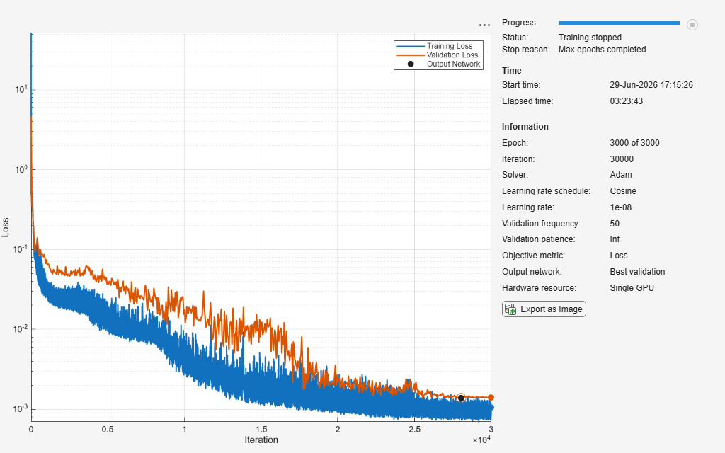
Train for 3000 epochs with a mini-batch size of 6.
Specify that the input and target data has the format "CSB" (channel, spatial, batch).
Monitor the training progress in a plot using the validation data and disable the verbose output.
Output the neural network with the lowest validation loss.

opts = trainingOptions("adam", ...
    LearnRateSchedule="cosine", ...
    MaxEpochs=3000, ...
    MiniBatchSize=6, ...
    InputDataFormats="CSB", ...
    TargetDataFormats="CSB", ...
    Plots="training-progress", ...
    ValidationData=cdsV, ...
    OutputNetwork="best-validation", ...
    Verbose=false);

Train Neural Network

Train the neural network with a custom loss function.

To encourage the neural network to match both the values and the spread of the target distribution, define a custom loss function weightedLoss that combines mean squared error with a variance penalty.

function loss = weightedLoss(Y,mask,T)

variancePenaltyWeight = 0.05;

totalNonPadding = sum(mask,"all");

lossMSE = sum(((Y - T).*mask).^2,"all") / totalNonPadding;

YMean = sum(Y.*mask,"all") / totalNonPadding;
TMean = sum(T.*mask,"all") / totalNonPadding;

YVariance = sum(((Y - YMean).*mask).^2,"all") / totalNonPadding;
TVariance = sum(((T - TMean).*mask).^2,"all") / totalNonPadding;

lossVariance = (YVariance - TVariance)^2;

loss = (1-variancePenaltyWeight)*lossMSE + variancePenaltyWeight*lossVariance;

end

Train the neural network using the trainnet function and the custom weighted loss function. By default, the trainnet function uses a GPU if one is available. Using a GPU requires a Parallel Computing Toolbox™ license and a supported GPU device. For information on supported devices, see GPU Computing Requirements (Parallel Computing Toolbox). Otherwise, the function uses the CPU. To choose the execution environment manually, use the ExecutionEnvironment training option.

Training a Transolver neural network can take a long time. It takes about 3 hours on a NVIDIA Titan RTX with 24GB of memory. By default, this example loads the network from a MAT file, attached to this example as a supporting file. To access this file, open the example as a live script. To retrain the neural network in this example, set the doTrain variable to true.

filenameNetwork = "electrostaticSimulationNetwork.mat";

if doTrain
    [net,info] = trainnet(cds,net,@weightedLoss,opts);
else
    load(filenameNetwork)
end

Visualize Neural Network Predictions

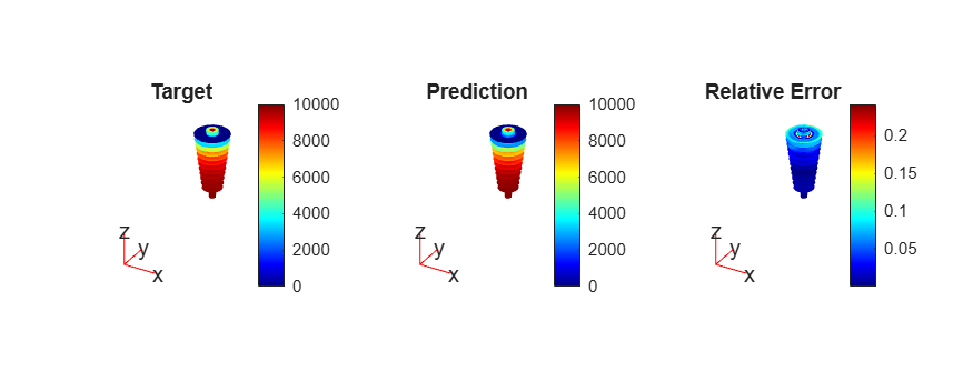
Visualize the neural network predictions by plotting the target potential, the predicted potential, and the relative error for a test observation.

Extract data from one of the test observations.

idx = 1;
D = data(idxTest(idx));

U = [
    D.Coord
    D.Epsilon'];

Preprocess the data using the same function used during training.

normU = preprocessElectrostaticInput(U, inputOffset, inputScale);

If a GPU is available, convert the data to gpuArray.

if canUseGPU
    normU = gpuArray(normU);
end

Make predictions using the Transolver neural network. Rescale the predictions using the training statistics.

V = predict(net,normU');
V = V.*outputScale + outputOffset;

To visualize only the bushing region, find the elements and nodes that belong to cell 2.

elementsBushing = findElements(D.Mesh,"Region",Cell=2);
nodesBushing = findNodes(D.Mesh,"Region",Cell=2);

Calculate the absolute and relative prediction errors.

absoluteError = abs(V-D.Potential);
relativeError = absoluteError./max(D.Potential(nodesBushing));

To set consistent color axis limits across the plots, compute the minimum and maximum potential values.

[minPotential, maxPotential] = bounds(D.Potential);

Visualize the predictions and errors using PDE plots.

h = figure;
h.Position(3) = 1.5*h.Position(3);
tiledlayout(1,3);
nexttile

pdeplot3D(D.Mesh.Nodes, ...
    D.Mesh.Elements(:,elementsBushing), ...
    ColorMapData=D.Potential);

title("Target");
clim([minPotential maxPotential]);

nexttile

pdeplot3D(D.Mesh.Nodes, ...
    D.Mesh.Elements(:,elementsBushing), ...
    ColorMapData=V)

title("Prediction");
clim([minPotential maxPotential]);
nexttile

pdeplot3D(D.Mesh.Nodes, ...
    D.Mesh.Elements(:,elementsBushing), ...
    ColorMapData=relativeError);

title("Relative Error")

Make Predictions With New Design

Use the Transolver neural network to predict the electric potential field for a new design geometry that the neural network did not see during training.

Load the stereolithography (STL) file representing the transformer bushing insulator geometry.

filename = "bushing_insulator_design.stl";
geometryBushing = fegeometry(filename);

Visualize the bushing insulator geometry.

figure
pdegplot(geometryBushing);
title("New Bushing Insulator Geometry");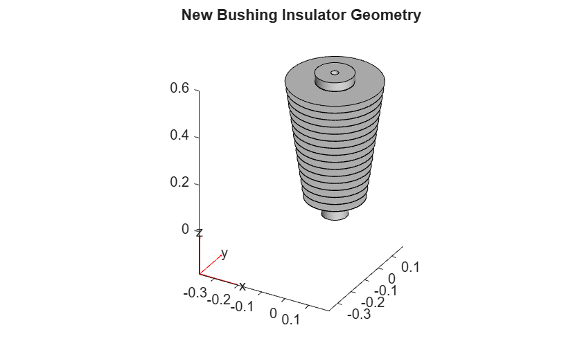

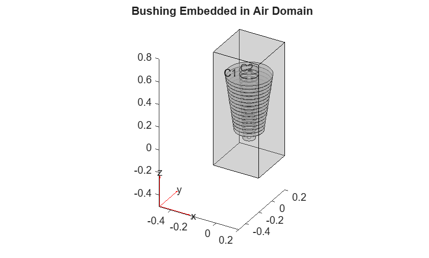
To model the electric field in the space surrounding the bushing, define a cuboid air domain that encloses the geometry.

geometryAir = multicuboid(0.4,0.4,1);
geometryAir = translate(geometryAir,[0 0 -0.2]);
geometryAir = fegeometry(geometryAir);

Combine the air and bushing geometries into a single model.

geometryModel = addCell(geometryAir,geometryBushing);

Visualize the combined geometry and inspect the cell labels. Cell 1 corresponds to the air domain and cell 2 corresponds to the bushing insulator.

figure

pdegplot(geometryModel, ...
    FaceAlpha=0.3, ...
    CellLabels="on");

title("Bushing Embedded in Air Domain")

Create an electrostatic finite element analysis (FEA) model.

model = femodel( ...        
    AnalysisType="electrostatic", ...
    Geometry=geometryModel);

Assign relative permittivity values based on the cell labels.

cellAir = 1;
cellBushing = 2;

model.MaterialProperties(cellAir) = materialProperties(RelativePermittivity=1);
model.MaterialProperties(cellBushing) = materialProperties(RelativePermittivity=5);

Set the vacuum permittivity to the physical constant $ε_{0} \approx 8.854 \times 1 0^{- 12}$ F/m.

model.VacuumPermittivity = 8.8541878128E-12;

To obtain a sufficiently fine mesh for accurate predictions, generate the mesh with a maximum element size of 0.025.

model = generateMesh(model,Hmax=0.025);

Prepare the inputs for the neural network.

Extract node coordinates and assign relative permittivity values to each node based on its region.

elementsBushing = findElements(model.Mesh,"Region",Cell=cellBushing);
nodesBushing = findNodes(model.Mesh,"Region",Cell=cellBushing);
nodesAir = findNodes(model.Mesh,"Region",Cell=cellAir);

coordinates = model.Mesh.Nodes;

To construct the input feature vector, assign relative permittivity values to each mesh node based on its cell region.

numNodes = size(model.Mesh.Nodes,2);
relativePermittivity = zeros(1,numNodes);
relativePermittivity(nodesAir) = model.MaterialProperties(cellAir).RelativePermittivity;
relativePermittivity(nodesBushing) = model.MaterialProperties(cellBushing).RelativePermittivity;

Concatenate the coordinates and material properties.

U = [
    coordinates
    relativePermittivity];

Preprocess the data using the same function used during training.

normU = preprocessElectrostaticInput(U, inputOffset, inputScale);

Make predictions using the Transolver neural network.

if canUseGPU
    normU = gpuArray(normU);
end

V = predict(net,normU');

Rescale predictions using the training statistics.

V = V.*outputScale + outputOffset;

Visualize the predictions in a PDE plot.

figure

pdeplot3D(model.Mesh.Nodes, ...
    model.Mesh.Elements(:,elementsBushing), ...
    ColorMapData=V);

title("Predictions")

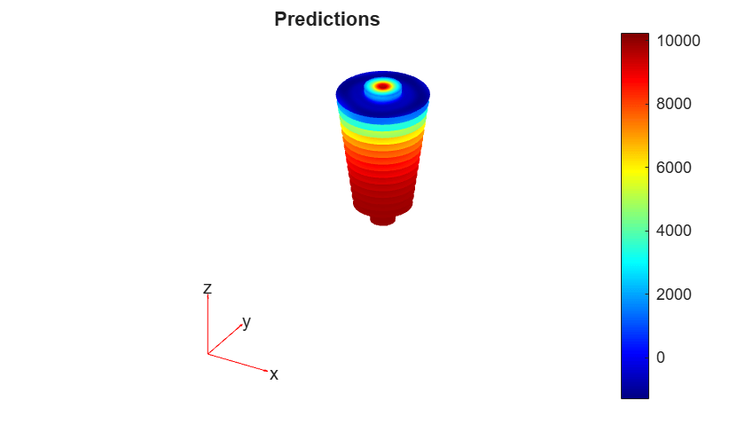
The plot shows the predicted electric potential on the bushing geometry. Values close to the lower end of the color spectrum indicate regions near ground potential. Values close to the upper end indicate regions at higher voltage.

Bibliography

Wu, Haixu, Huakun Luo, Haowen Wang, Jianmin Wang, and Mingsheng Long. “Transolver: A Fast Transformer Solver for PDEs on General Geometries.” arXiv.Org, February 4, 2024. https://arxiv.org/abs/2402.02366v2.