Train a Twin Network for Dimensionality Reduction

Load and Preprocess Training Data

Load the training data, which consists of images of handwritten digits. The function digitTrain4DArrayData loads the digit images and their labels.

[XTrain,TTrain] = digitTrain4DArrayData;

XTrain is a 28-by-28-by-1-by-5000 array containing 5000 single-channel images, each of size 28-by-28. The values of each pixel are between 0 and 1. TTrain is a categorical vector containing the labels for each observation, which are the numbers from 0 to 9 corresponding to the value of the written digit.

Display a random selection of the images.

perm = randperm(numel(TTrain),9);
imshow(imtile(XTrain(:,:,:,perm),ThumbnailSize=[100 100]));

Create Pairs of Similar and Dissimilar Images

To train the network, the data must be grouped into pairs of images that are either similar or dissimilar. Here, similar images are defined as having the same label, while dissimilar images have different labels. The function getTwinBatch (defined in the Supporting Functions section of this example) creates randomized pairs of similar or dissimilar images, pairImage1 and pairImage2. The function also returns the label pairLabel, which identifies if the pair of images is similar or dissimilar to each other. Similar pairs of images have pairLabel = 1, while dissimilar pairs have pairLabel = 0.

As an example, create a small representative set of five pairs of images

batchSize = 10;
[pairImage1,pairImage2,pairLabel] = getTwinBatch(XTrain,TTrain,batchSize);

Display the generated pairs of images.

figure
tiledlayout("flow")
for i = 1:batchSize
    nexttile
    imshow([pairImage1(:,:,:,i) pairImage2(:,:,:,i)]);
    if pairLabel(i) == 1
        s = "similar";
    else
        s = "dissimilar";
    end
    title(s)
end

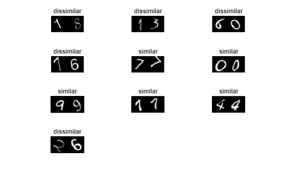
In this example, a new batch of 180 paired images is created for each iteration of the training loop. This ensures that the network is trained on a large number of random pairs of images with approximately equal proportions of similar and dissimilar pairs.

Define Network Architecture

The twin network architecture is illustrated in the following diagram.

In this example, the two identical subnetworks are defined as a series of fully connected layers with ReLU layers. Create a network that accepts 28-by-28-by-1 images and outputs the two feature vectors used for the reduced feature representation. The network reduces the dimensionality of the input images to two, a value that is easier to plot and visualize than the initial dimensionality of 784.

For the first two fully connected layers, specify an output size of 1024 and use the He weight initializer.

For the final fully connected layer, specify an output size of two and use the He weights initializer.

layers = [
    imageInputLayer([28 28],Normalization="none")
    fullyConnectedLayer(1024,WeightsInitializer="he")
    reluLayer
    fullyConnectedLayer(1024,WeightsInitializer="he")
    reluLayer
    fullyConnectedLayer(2,WeightsInitializer="he")];

To train the network with a custom training loop and enable automatic differentiation, convert the layer array to a dlnetwork object.

net = dlnetwork(layers);

Define Model Loss Function

Create the function modelLoss (defined in the Supporting Functions section of this example). The modelLoss function takes the twin dlnetwork object net and a mini-batch of input data X1 and X2 with their labels pairLabels. The function returns the loss values and the gradients of the loss with respect to the learnable parameters of the network.

The objective of the twin network is to output a feature vector for each image such that the feature vectors are similar for similar images, and notably different for dissimilar images. In this way, the network can discriminate between the two inputs.

Find the contrastive loss between the outputs from the last fully connected layer, the feature vectors features1 and features1 from pairImage1 and pairImage2, respectively. The contrastive loss for a pair is given by [3]

where $\mathit{y}$ is the value of the pair label ($\mathit{y}=1$ for similar images;$\mathit{y}=0$ for dissimilar images), and $\mathit{d}$ is the Euclidean distance between two features vectors $\mathit{f1}$ and $\mathit{f2}$: $\mathit{d}={\Vert \mathit{f1}-\mathit{f2}\Vert }_2$.

The $margin$ parameter is used for constraint: if two images in a pair are dissimilar, then their distance should be at least $margin$, or a loss will be incurred.

The contrastive loss has two terms, but only one is ever non-zero for a given image pair. In the case of similar images, the first term can be non-zero and is minimized by reducing the distance between the image features $\mathit{f1}$ and $\mathit{f2}$. In the case of dissimilar images, the second term can be non-zero, and is minimized by increasing the distance between the image features, to at least a distance of $margin$. The smaller the value of $margin$, the less constraining it is over how close a dissimilar pair can be before a loss is incurred.

Specify Training Options

Specify the value of $margin$ to use during training.

margin = 0.3;

Specify the options to use during training. Train for 3000 iterations.

numIterations = 3000;
miniBatchSize = 180;

Specify the options for Adam optimization:

learningRate = 1e-4;
trailingAvg = [];
trailingAvgSq = [];
gradDecay = 0.9;
gradDecaySq = 0.99;

Train Model

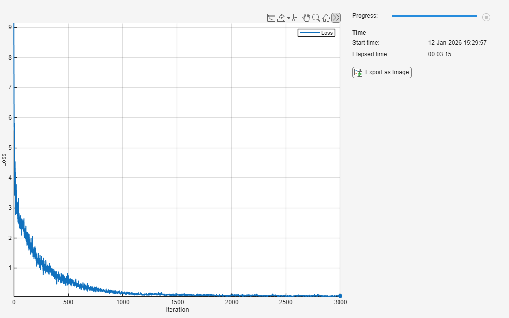
Train the model using a custom training loop.

Initialize the TrainingProgressMonitor object. Because the timer starts when you create the monitor object, make sure that you create the object close to the training loop.

monitor = trainingProgressMonitor(Metrics="Loss",XLabel="Iteration");

Loop over the training data and update the network parameters at each iteration. For each iteration:

iteration = 0;
% Loop over mini-batches.
while iteration < numIterations && ~monitor.Stop
    iteration = iteration + 1;

    % Extract mini-batch of image pairs and pair labels
    [X1,X2,pairLabels] = getTwinBatch(XTrain,TTrain,miniBatchSize);

    % Convert mini-batch of data to dlarray. Specify the dimension labels
    % "SSCB" (spatial, spatial, channel, batch) for image data
    X1 = dlarray(single(X1),"SSCB");
    X2 = dlarray(single(X2),"SSCB");

    % If training on a GPU, then convert data to gpuArray.
    if canUseGPU
        X1 = gpuArray(X1);
        X2 = gpuArray(X2);
    end

    % Evaluate the model loss and gradients using dlfeval and the modelLoss
    % function listed at the end of the example.
    [loss,gradients] = dlfeval(@modelLoss,net,X1,X2,pairLabels,margin);

    % Update the twin network parameters.
    [net,trailingAvg,trailingAvgSq] = adamupdate(net,gradients, ...
        trailingAvg,trailingAvgSq,iteration,learningRate,gradDecay,gradDecaySq);

    % Update the training progress monitor.
    recordMetrics(monitor,iteration,Loss=loss);
    monitor.Progress = 100 * iteration/numIterations;
end

Visualize Image Similarities

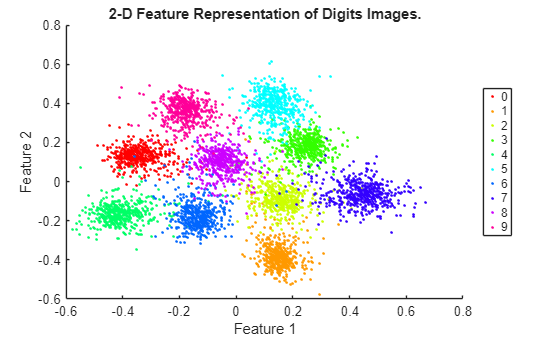
To evaluate how well the network is doing at dimensionality reduction, compute and plot the reduced features of a set of test data. Load the test data, which consists of images of handwritten digits similar to the training data. Convert the test data to dlarray and specify the dimension labels "SSCB" (spatial, spatial, channel, batch). If you are using a GPU, convert the test data to gpuArray.

[XTest,TTest] = digitTest4DArrayData;
XTest = dlarray(single(XTest),"SSCB");

if canUseGPU
    XTest = gpuArray(XTest);
end

Compute the reduced features of the test data.

FTest = predict(net,XTest);

For each group, plot the first two reduced features of the test data.

uniqueGroups = unique(TTest);
colors = hsv(length(uniqueGroups));

figure
hold on
for k = 1:length(uniqueGroups)
    ind = TTest==uniqueGroups(k);

    plot(FTest(1,ind),FTest(2,ind),".",Color=colors(k,:));
end
hold off

xlabel("Feature 1")
ylabel("Feature 2")
title("2-D Feature Representation of Digits Images.");

legend(uniqueGroups,Location="eastoutside");

Use the Trained Network to Find Similar Images

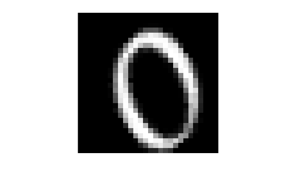
You can use the trained network to find a selection of images that are similar to each other out of a group. Extract a single test image from the test data and display it.

testIdx = randi(5000);
testImg = XTest(:,:,:,testIdx);

trialImgDisp = extractdata(testImg);

figure
imshow(trialImgDisp,InitialMagnification=500);

Create a group of images containing the test data but does not include the extracted test image.

groupX = XTest;
groupX(:,:,:,testIdx) = [];

Find the reduced features of the test image using predict.

trialF = predict(net,testImg);

Find the 2-D reduced feature representation of each of the images in the group using the trained network.

FGroupX = predict(net,groupX);

Use the reduced feature representation to find the nine images in the group that are closest to the test image, using the Euclidean distance metric. Display the images.

distances = vecnorm(extractdata(trialF - FGroupX));
[~,idx] = sort(distances);
sortedImages = groupX(:,:,:,idx);
sortedImages = extractdata(sortedImages);

figure
imshow(imtile(sortedImages(:,:,:,1:9)),InitialMagnification=500);

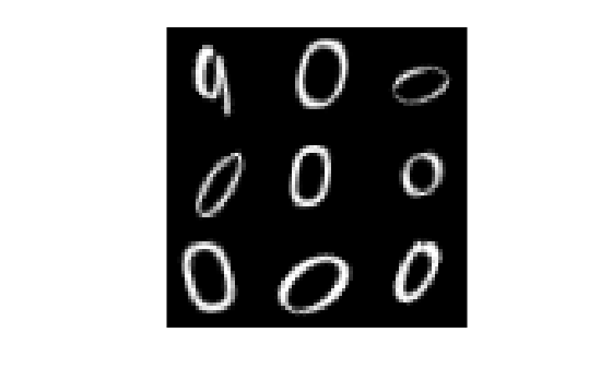
By reducing the images to a lower dimensionality, the network is able to identify images that are similar to the trial image. The reduced feature representation allows the network to discriminate between images that are similar and dissimilar. Twin networks are often used in the context of facial or signature recognition. For example, you can train a twin network to accept an image of a face as an input, and return a set of the most similar faces from a database.

Supporting Functions

Model Loss Function

The function modelLoss takes the twin dlnetwork object net, a pair of mini-batch input data X1 and X2, and the label pairLabels. The function returns the contrastive loss between the reduced dimensionality features of the paired images and the gradients of the loss with respect to the learnable parameters in the network. Within this example, the function modelLoss is introduced in the section Define Model Loss Function.

function [loss,gradients] = modelLoss(net,X1,X2,pairLabel,margin)
% The modelLoss function calculates the contrastive loss between the
% paired images and returns the loss and the gradients of the loss with
% respect to the network learnable parameters

% Pass first half of image pairs forward through the network
F1 = forward(net,X1);
% Pass second set of image pairs forward through the network
F2 = forward(net,X2);

% Calculate contrastive loss
loss = contrastiveLoss(F1,F2,pairLabel,margin);

% Calculate gradients of the loss with respect to the network learnable
% parameters
gradients = dlgradient(loss,net.Learnables);

end

function loss = contrastiveLoss(F1,F2,pairLabel,margin)
% The contrastiveLoss function calculates the contrastive loss between
% the reduced features of the paired images

% Define small value to prevent taking square root of 0
delta = 1e-6;

% Find Euclidean distance metric
distances = sqrt(sum((F1 - F2).^2,1) + delta);

% label(i) = 1 if features1(:,i) and features2(:,i) are features
% for similar images, and 0 otherwise
lossSimilar = pairLabel.*(distances.^2);

lossDissimilar = (1 - pairLabel).*(max(margin - distances, 0).^2);

loss = 0.5*sum(lossSimilar + lossDissimilar,"all");

end

Create Batches of Image Pairs

The following functions create randomized pairs of images that are similar or dissimilar, based on their labels. Within this example, the function getTwinBatch is introduced in the section Create Pairs of Similar and Dissimilar Images.

function [X1,X2,pairLabels] = getTwinBatch(X,Y,miniBatchSize)
% getTwinBatch returns a randomly selected batch of paired images.
% On average, this function produces a balanced set of similar and
% dissimilar pairs.
pairLabels = zeros(1, miniBatchSize);
imgSize = size(X(:,:,:,1));
X1 = zeros([imgSize 1 miniBatchSize]);
X2 = zeros([imgSize 1 miniBatchSize]);

for i = 1:miniBatchSize
    choice = rand(1);
    if choice < 0.5
        [pairIdx1, pairIdx2, pairLabels(i)] = getSimilarPair(Y);
    else
        [pairIdx1, pairIdx2, pairLabels(i)] = getDissimilarPair(Y);
    end
    X1(:,:,:,i) = X(:,:,:,pairIdx1);
    X2(:,:,:,i) = X(:,:,:,pairIdx2);
end

end

function [pairIdx1,pairIdx2,pairLabel] = getSimilarPair(classLabel)
% getSimilarPair returns a random pair of indices for images
% that are in the same class and the similar pair label = 1.

% Find all unique classes.
classes = unique(classLabel);

% Choose a class randomly which will be used to get a similar pair.
classChoice = randi(numel(classes));

% Find the indices of all the observations from the chosen class.
idxs = find(classLabel==classes(classChoice));

% Randomly choose two different images from the chosen class.
pairIdxChoice = randperm(numel(idxs),2);
pairIdx1 = idxs(pairIdxChoice(1));
pairIdx2 = idxs(pairIdxChoice(2));
pairLabel = 1;
end

function  [pairIdx1,pairIdx2,pairLabel] = getDissimilarPair(classLabel)
% getDissimilarPair returns a random pair of indices for images
% that are in different classes and the dissimilar pair label = 0.

% Find all unique classes.
classes = unique(classLabel);

% Choose two different classes randomly which will be used to get a dissimilar pair.
classesChoice = randperm(numel(classes), 2);

% Find the indices of all the observations from the first and second classes.
idxs1 = find(classLabel==classes(classesChoice(1)));
idxs2 = find(classLabel==classes(classesChoice(2)));

% Randomly choose one image from each class.
pairIdx1Choice = randi(numel(idxs1));
pairIdx2Choice = randi(numel(idxs2));
pairIdx1 = idxs1(pairIdx1Choice);
pairIdx2 = idxs2(pairIdx2Choice);
pairLabel = 0;
end

References

Bromley, J., I. Guyon, Y. LeCun, E. Säckinger, and R. Shah. "Signature Verification using a "Siamese" Time Delay Neural Network." In Proceedings of the 6th International Conference on Neural Information Processing Systems (NIPS 1993), 1994, pp737-744. Available at Signature Verification using a "Siamese" Time Delay Neural Network on the NeurIPS Proceedings website.
Wenpeg, Y., and H Schütze. "Convolutional Neural Network for Paraphrase Identification." In Proceedings of 2015 Conference of the North American Chapter of the ACL, 2015, pp901-911. Available at Convolutional Neural Network for Paraphrase Identification on the ACL Anthology website.
Hadsell, R., S. Chopra, and Y. LeCun. "Dimensionality Reduction by Learning an Invariant Mapping." In Proceedings of the 2006 IEEE Computer Society Conference on Computer Vision and Pattern Recognition (CVPR 2006), 2006, pp1735-1742.
See Also
dlarray | dlgradient | dlfeval | dlnetwork | adamupdate