Incorporate Macroeconomic Scenario Projections in Loan Portfolio ECL Calculations
This example shows how to generate macroeconomic scenarios and perform expected credit loss (ECL) calculations for a portfolio of loans. The workflow in this example shows important computational steps required to estimate provisions for credit losses following regulations such as IFRS 9 or CECL. In practice, the determination of loan provisions is a much more involved operational program requiring the collaboration of multiple departments in an institution. The goal of this example is to show useful computational tools that can support this process.
This example includes two parts:
Part 1 produces macroeconomic scenarios for the credit analysis and fits a vector autoregression (VAR) model to macroeconomic data. The workflow describes three qualitative scenario narratives with selected macro projections covering a few quarters ahead. It uses the conditional forecasting capabilities of the fitted VAR model to generate longer term projections for the macroeconomic variables.
Part 2 focuses on the credit analysis of an existing portfolio of loans. It uses three existing credit models are used, namely, a lifetime probability of default (PD) model, a loss given default (LGD) model, and an exposure at default (EAD) model. These models predict lifetime PD, LGD, and EAD values several periods ahead, given projections on loan-specific predictor variables and the macroeconomic scenarios from Part 1. The workflow estimates the loan loss provisions using the
portfolioECLfunction, given the marginal PD, LGD, and EAD projections for different scenarios.
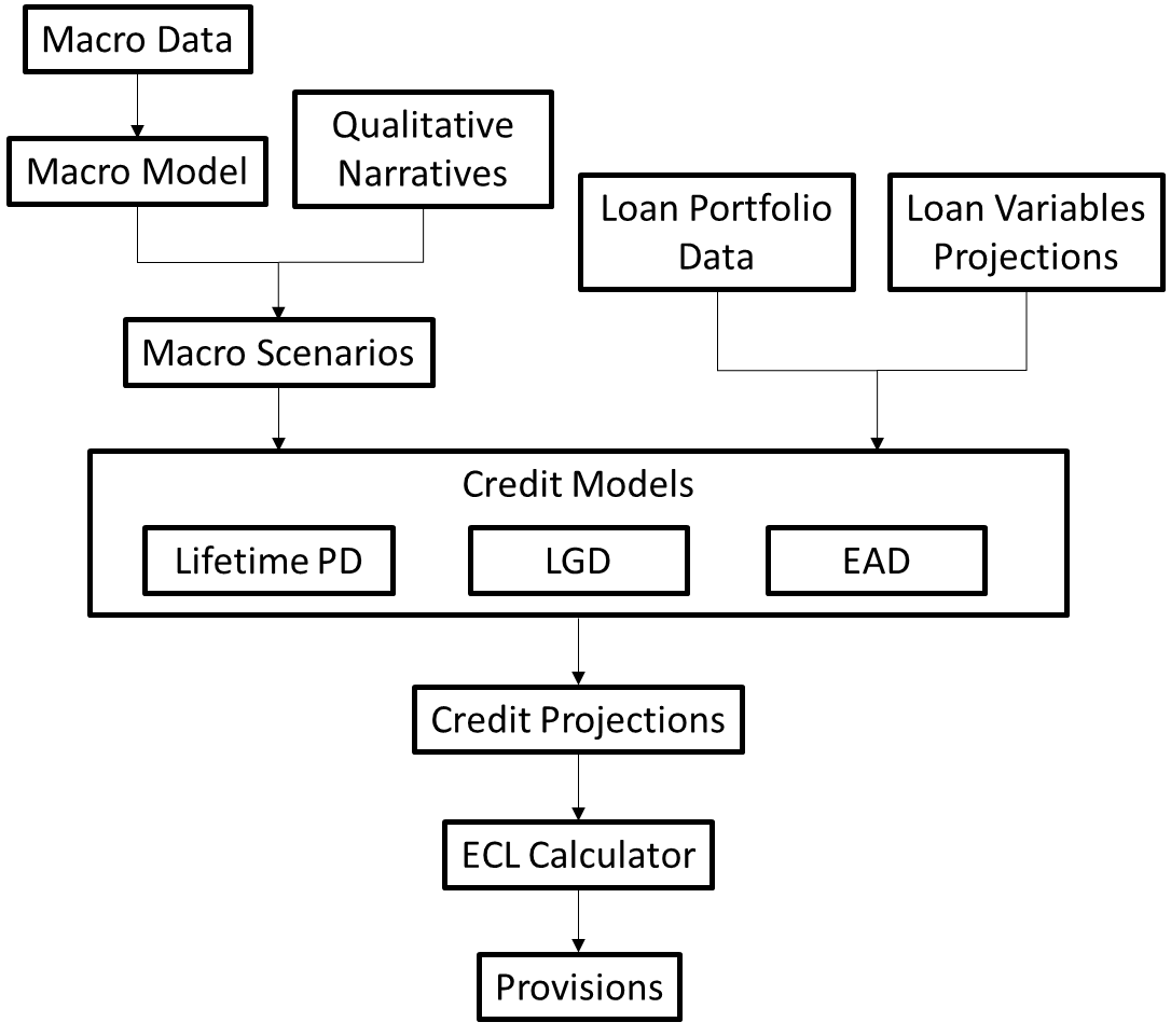
The following diagram summarizes the workflow in this example.
Part 1: Macroeconomic Scenarios
This part of the example shows how to fit an econometric model and how to use the fitted model with hypothesized conditions to produce macroeconomic scenarios.
In practice, the determination and approval of macroeconomic scenarios is an involved process. Institutions source macroeconomic scenarios from external vendors or they maintain internal macroeconomic models and produce scenarios. An institution can have existing models to generate scenarios, which are reviewed and updated infrequently. Some macroeconomic model developers use econometric models, while others prefer to explore alternative statistical models, such as machine learning or deep learning models. For more details, see Train Deep Neural Networks (Deep Learning Toolbox).
For concreteness, the example fits a vector autoregressive (VAR) econometric model. For alternative econometric models, such as Vector Error-Correction Models, see the example, Model the United States Economy. Also, the Econometric Modeler enables you to interactively fit and analyze econometric models, including VAR and VEC models. For alternative time series modeling techniques, see Statistical and Machine Learning Toolbox™ and Deep Learning Toolbox™.
Part 1 describes the following workflow:
This example uses the Data_USEconModel.mat data set included with Econometrics Toolbox. The data set includes several macroeconomic variables measured quarterly from March, 1947, through March, 2009 (near the start of the global financial crisis). For more details on the series, inspect the Description variable in the data file.
The measurements help emphasize the sensitivity of the credit projections to stressed macroeconomic conditions. You can apply the steps in this example to fit macroeconomic models using recent data.
Visualize and Transform Data
This example includes the following variables in the model:
GDP: Gross domestic productUNRATE: Unemployment rateTB3MS: Three-month treasury bill yield
The variables sufficiently determine scenarios for the credit models in Part 2 of this example. However, the model can include additional variables, for example, variables that can explain the dynamics of the economy enough to improve model predictions.
Load the data. Visualize the raw macroeconomic time series.
load Data_USEconModel
varnames = ["GDP" "UNRATE" "TB3MS"];
DataMacro = rmmissing(DataTimeTable(:,varnames));  % Remove initial rows with UNRATE = NaN
DataMacro.Time.Format = "default";

figure
t = tiledlayout(3,1);
nexttile
plot(DataMacro.Time,DataMacro.GDP)
title("GDP")
nexttile
plot(DataMacro.Time,DataMacro.UNRATE)
title("UNRATE")
nexttile
plot(DataMacro.Time,DataMacro.TB3MS)
title("TB3MS")
title(t,"Macroeconomic Time Series")

All series appear nonstationary and have different scales. Because model estimation with nonstationary variables is problematic (see Time Series Regression IV: Spurious Regression), transform each series appropriately.
The GDP series shows exponential growth and has a larger scale than the other variables. Because GDP percent growth from quarter to quarter is common to report, is close in scale to the other variables, and is required by the credit models in Part 2, try to stabilize the series by computing its percent returns.
The unemployment and interest rate series do not show exponential growth, but they appear to have a stochastic trend. You can stabilize the series by applying the first difference to each. The credit models in Part 2 use the original units of these series; you can back-transform the series to their original units for the credit analysis.
Transform each series, and plot the results. Include the transformed variables in the timetable, prepad each transformation with NaN to synchronize the series (the first difference operation of a series results in one less observation).
DataMacro.GDPGROWTH = 100*[NaN; price2ret(DataMacro.GDP)];  % Growth rate in percent
DataMacro.UNRATEDIFF = [NaN; diff(DataMacro.UNRATE)];
DataMacro.TB3MSDIFF = [NaN; diff(DataMacro.TB3MS)];
DataMacro = rmmissing(DataMacro);                           % Remove initial missing values
numObs = height(DataMacro);

figure
t = tiledlayout(3,1);
nexttile
plot(DataMacro.Time,DataMacro.GDPGROWTH)
yline(0)
title("GDPGROWTH")
nexttile
plot(DataMacro.Time,DataMacro.UNRATEDIFF)
yline(0)
title("UNRATEDIFF")
nexttile
plot(DataMacro.Time,DataMacro.TB3MSDIFF)
yline(0)
title("TB3MSDIFF")
title(t,"Transformed Macroeconomic Series")
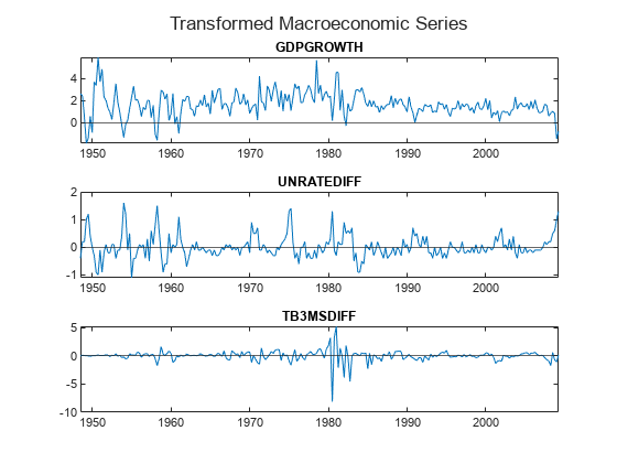
The series appear stable. To confirm the visual conclusions, conduct stationarity tests on each series.
Conduct Stationarity Tests and Select Model Lags
To fit a VAR model, all variables must be stationarity. Econometrics Toolbox includes several tests for stationarity; see Unit Root Tests.
This example uses the augmented Dickey-Fuller (ADF) test for unit root nonstationarity (see adftest). The null hypothesis of the test is that the input series is unit root nonstationary. Specified options determine the alternative hypothesis. The Model option of the ADF test specifies the dynamic structure of the alternative model for the test variable, specifically, autoregressive AR, autoregressive with drift ARD, or trend-stationary TS. The Lags option specifies the number of AR lags in the alternative model, specifically, the number where (the value of the series periods back) influences the evolution of the series to the current step . The ADF test results give information on whether the series is stationarity and on the structure of the autoregressive model that is appropriate for the series.
Use the ADF test to assess whether each series is stationary and to determine the appropriate dynamic model with number of lags for each series. The drop-down controls enable you to set model choices and variables for the ADF test. The adftest call runs separate tests from lags 0 through 4. The current settings in the code assesses whether TB3MSDIFF is stationary, assuming an ARD model.
ADFModelChoice ="ARD"; DataVariableChoice =
"TB3MSDIFF"; ADFTbl = adftest(DataMacro,'model',ADFModelChoice,'Lags',0:4,'DataVariable',DataVariableChoice)
ADFTbl=5×8 table
                h      pValue     stat      cValue     Lags    Alpha     Model      Test
              _____    ______    _______    _______    ____    _____    _______    ______

    Test 1    true     0.001     -17.668    -2.8738     0      0.05     {'ARD'}    {'T1'}
    Test 2    true     0.001       -14.8    -2.8738     1      0.05     {'ARD'}    {'T1'}
    Test 3    true     0.001     -8.3548    -2.8739     2      0.05     {'ARD'}    {'T1'}
    Test 4    true     0.001     -7.6124    -2.8739     3      0.05     {'ARD'}    {'T1'}
    Test 5    true     0.001     -6.0646     -2.874     4      0.05     {'ARD'}    {'T1'}
ADFTbl is a table containing the results of all conducted tests for assessing whether TB3MSDIFF is stationary. Each row is a separate test for each lag in the Lags variable. Values of h indicate whether to reject the null hypothesis at Alpha level of significance. Small enough p-values in the pValue variable suggest whether to reject the null hypothesis. h = 1 suggests to reject the null hypothesis in favor of the alternative, and h = 0 suggests failure to reject the null hypothesis. In this case, h = 1 for all lags, so there is evidence that the TB3MSDIFF series is a stationary, autoregressive process with drift among all lags.
For each untransformed and transformed series in this example, use the drop-down controls to assess whether the series is unit root nonstationary against each alternative model including the AR lags 1 through 4.
The results are as follows:
GDP: The ADF test fails to reject the null hypothesis for all settings. Exclude this series from the VAR model.GDPGROWTH: The ADF test rejects the null hypothesis for all settings. Include this series in the VAR model.UNRATE: The tests return mixed results. The tests that use anARDalternative model with lags 1 through 3 reject the null hypothesis. Therefore, the unemployment rate does not require transforming because it has a deterministic trend. Include the raw series in the VAR model with a drift term. Also, use of the raw series is convenient because the series does not need to be back-transformed; it simplifies the scenario determination.TB3MS: The ADF test fails to reject the null hypothesis for all settings. Exclude this series from the VAR model.TB3MSDIFF: The ADF test rejects the null hypothesis for all settings. Include this series in the VAR model.
In addition to using ADF test results, you can determine the number of lags by using Akaike information criterion (AIC), Bayesian information criterion (BIC), and likelihood ratio tests. For an example, see Select Appropriate Lag Order. These approaches are useful, but they have caveats (for example, they are sensitive to the scaling of the series).
This example proceeds using two lags, which is reasonable from an application standpoint (it specifies to include information up to two quarters back). It leads to a less complex model, which is easier to analyze.
Fit VAR Model
Fit a VAR model that includes the GDP growth, unemployment rate, and the first difference of the interest rate time series as endogenous variables. Include two AR lags in the model. For details, see varm and estimate.
varnames = ["GDPGROWTH" "UNRATE" "TB3MSDIFF"];
numVars = length(varnames);
numLags = 2;

% 3-D VAR(2) model template
Mdl = varm(numVars,numLags);
Mdl.SeriesNames = varnames;

% Fit the model
[MacroVARModel,~,~,Residuals] = estimate(Mdl,DataMacro{:,varnames});
Visualize the fitted values for each series by using the drop-down control.
numRes = size(Residuals,1); DataMacro.GDPGROWTH_Predicted = NaN(numObs,1); DataMacro.GDPGROWTH_Predicted(end-numRes+1:end) = DataMacro.GDPGROWTH(end-numRes+1:end) - Residuals(:,1); DataMacro.UNRATE_Predicted = NaN(numObs,1); DataMacro.UNRATE_Predicted(end-numRes+1:end) = DataMacro.UNRATE(end-numRes+1:end) - Residuals(:,2); DataMacro.TB3MSDIFF_Predicted = NaN(numObs,1); DataMacro.TB3MSDIFF_Predicted(end-numRes+1:end) = DataMacro.TB3MSDIFF(end-numRes+1:end) - Residuals(:,3); PlotVariableChoice ="GDPGROWTH"; figure plot(DataMacro.Time,DataMacro.(PlotVariableChoice)) hold on plot(DataMacro.Time,DataMacro.(strcat(PlotVariableChoice,"_Predicted")),"-.") hold off title(strcat("Model Fit ",PlotVariableChoice)) ylabel(PlotVariableChoice) legend("Observed","Predicted") grid on
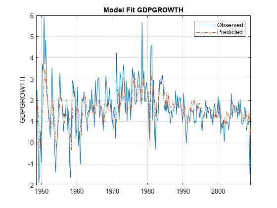
The model seems to have less variability than the actual data; the fitted values do not seem to go as high or as low as the most extreme values in the data. This result suggests the model error is smaller for small to medium GDP changes, but the errors are larger for more extreme GDP changes. Therefore, you can expect the model residuals to show heavy tails. A thorough analysis of residuals and autocorrelation is out of the scope of this example. For more details, see Time Series Regression VI: Residual Diagnostics. This observation means the model seems more reliable for forecasts, which work with expected values (central tendencies around current levels), and less reliable for analyses of tail behavior (very extreme shocks away from current levels).
A review of model coefficients is an important model validation step. The way the series and their lagged information influence the latest values of the series should have a reasonable explanation.
Display the estimated coefficients and inferences.
summarize(MacroVARModel)
   AR-Stationary 3-Dimensional VAR(2) Model

    Effective Sample Size: 242
    Number of Estimated Parameters: 21
    LogLikelihood: -681.275
    AIC: 1404.55
    BIC: 1477.82

                     Value      StandardError    TStatistic      PValue
                   _________    _____________    __________    __________

    Constant(1)    -0.010079       0.26158        -0.03853        0.96926
    Constant(2)       0.3433      0.099669          3.4444     0.00057241
    Constant(3)      0.11773       0.25581         0.46024        0.64535
    AR{1}(1,1)       0.32725      0.073009          4.4823     7.3852e-06
    AR{1}(2,1)     -0.071852      0.027819         -2.5829      0.0097982
    AR{1}(3,1)      0.098221        0.0714          1.3756        0.16893
    AR{1}(1,2)      -0.22429       0.19147         -1.1714        0.24145
    AR{1}(2,2)        1.4205      0.072958           19.47     1.9537e-84
    AR{1}(3,2)      -0.50519       0.18725         -2.6979      0.0069782
    AR{1}(1,3)      0.092278      0.067309           1.371        0.17039
    AR{1}(2,3)      0.040064      0.025647          1.5621        0.11825
    AR{1}(3,3)      -0.30309      0.065826         -4.6045     4.1352e-06
    AR{2}(1,1)       0.15851      0.063174           2.509       0.012107
    AR{2}(2,1)      0.016333      0.024071         0.67854        0.49743
    AR{2}(3,1)       0.10361      0.061782          1.6771       0.093525
    AR{2}(1,2)       0.37458       0.19298           1.941       0.052255
    AR{2}(2,2)       -0.4632      0.073531         -6.2994     2.9882e-10
    AR{2}(3,2)       0.42524       0.18873          2.2532       0.024246
    AR{2}(1,3)      -0.15819        0.0655         -2.4152       0.015728
    AR{2}(2,3)       0.03071      0.024957          1.2305        0.21851
    AR{2}(3,3)       -0.3519      0.064056         -5.4936      3.939e-08


   Innovations Covariance Matrix:
    0.8575   -0.1668    0.2065
   -0.1668    0.1245   -0.1156
    0.2065   -0.1156    0.8201


   Innovations Correlation Matrix:
    1.0000   -0.5103    0.2463
   -0.5103    1.0000   -0.3616
    0.2463   -0.3616    1.0000
For example, for GDP growth, the diagonal coefficients are positive, with the first lag coefficient about twice as large as the second lag coefficient. This result means there is some inertia in the GDP series, some positive memory, and the more recent quarter has more influence than the growth two periods ago. For unemployment, the first lag diagonal coefficient is positive (and relatively large), but the second lag coefficient is negative. This result suggests that there is strong inertia for unemployment with respect to the previous quarter, but that there is a rebound effect with respect to two quarters before. Expert judgment is required to analyze model coefficients and raise flags in unexpected situations (a thorough analysis of the model coefficients and their especially statistical significance are beyond the scope of this example).
Define Macroeconomic Scenarios
Econometric model forecasts use the model parameters and recent observations of the time series to make predictions. The model forecast is a natural candidate for a macroeconomic scenario. However, the data and the model fully determine the forecasts, without qualitative views.
Forecast the estimated VAR model into a 30-period horizon by using forecast. Initialize the forecasts by specifying the estimation data as a presample.
NumPeriods = 30;
ModelForecast = forecast(MacroVARModel,NumPeriods,DataMacro{:,varnames});
For later use by models and visualizations, append the latest observed quarter.
ModelForecast = [DataMacro{end,varnames}; ModelForecast];
fhTime = dateshift(DataMacro.Time(end),"end","quarter",0:NumPeriods)
fhTime = 1×31 datetime
31-Mar-2009 30-Jun-2009 30-Sep-2009 31-Dec-2009 31-Mar-2010 30-Jun-2010 30-Sep-2010 31-Dec-2010 31-Mar-2011 30-Jun-2011 30-Sep-2011 31-Dec-2011 31-Mar-2012 30-Jun-2012 30-Sep-2012 31-Dec-2012 31-Mar-2013 30-Jun-2013 30-Sep-2013 31-Dec-2013 31-Mar-2014 30-Jun-2014 30-Sep-2014 31-Dec-2014 31-Mar-2015 30-Jun-2015 30-Sep-2015 31-Dec-2015 31-Mar-2016 30-Jun-2016 30-Sep-2016
TTForecast = array2timetable(ModelForecast,RowTimes=fhTime,VariableNames=varnames);
The model forecasts interest rate changes to TB3MSDIFF. Postprocess the forecast to recover the predicted values for the interest rate in TB3MS.
TTForecast.TB3MS = TTForecast.TB3MSDIFF;
TTForecast.TB3MS(1) = DataMacro.TB3MS(end);
TTForecast.TB3MS = cumsum(TTForecast.TB3MS)
TTForecast=31×4 timetable
       Time        GDPGROWTH    UNRATE    TB3MSDIFF     TB3MS
    ___________    _________    ______    _________    ________

    31-Mar-2009    -0.78191        8.5         0.18        0.21
    30-Jun-2009     0.47974      9.088      -1.0128    -0.80284
    30-Sep-2009      1.0466     9.2336     -0.64918      -1.452
    31-Dec-2009       1.842     9.1257     0.023293     -1.4287
    31-Mar-2010      2.2753     8.8953    -0.055275      -1.484
    30-Jun-2010      2.4409     8.6173    -0.072599     -1.5566
    30-Sep-2010      2.5506     8.3213     0.063912     -1.4927
    31-Dec-2010      2.5904     8.0292     0.087927     -1.4048
    31-Mar-2011       2.556     7.7556     0.069531     -1.3352
    30-Jun-2011      2.4975     7.5053     0.081449     -1.2538
    30-Sep-2011      2.4306       7.28     0.085102     -1.1687
    31-Dec-2011      2.3547     7.0803     0.074533     -1.0942
    31-Mar-2012      2.2781     6.9051     0.067146      -1.027
    30-Jun-2012      2.2065     6.7522     0.061337    -0.96567
    30-Sep-2012      2.1401     6.6197     0.053405    -0.91227
    31-Dec-2012      2.0797     6.5054     0.045859    -0.86641
      ⋮
Visualize each model forecast by using the drop-down control.
VarToPlot ="UNRATE"; figure plot(DataMacro.Time,DataMacro{:,VarToPlot}) hold on plot(TTForecast.Time,TTForecast{:,VarToPlot},"--") yline(0) hold off title(VarToPlot) legend("Data","Forecast")
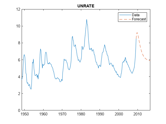
The GDP growth reverts quickly to the average levels, with one more quarter of economic contraction, and growth rates over 1% by the third quarter.
The unemployment rate peaks at just over 9% and then goes back to average levels, at a slower pace than the GDP.
The model forecast predicts significantly negative interest rates going forward for a long period of time.
To define the scenarios for the credit analysis in Part 2, this example uses scenario narratives with qualitative views up to a few quarters ahead. This example combines the scenario narratives with conditional forecasting of the model to extend the predictions to several years ahead, where the predicted values revert to long-term levels. This approach can determine values for variables not described in the narrative, but are included in the macroeconomic model. For example, if only the GDP growth and unemployment rate are in the narrative, the corresponding interest rate scenario can be determined with conditional forecasting.
This example explores three scenarios: slow recovery, baseline, and fast recovery.
Slow Recovery Scenario
In this scenario, the GDP contracts for four more quarters, with a maximum contraction of 1.5% one quarter ahead. The unemployment rate peaks at 11% three quarters ahead. The interest rate remains negative for four quarters.
Forecast the model under this scenario. Preprocess the raw interest rate series of the estimated model, then postprocess their forecasts to the original units.
TTSlow = TTForecast; % Initialize forecast variables

TTSlow.GDPGROWTH(2:7) = [-1.5; -1.2; -0.8; -0.3; 0.1; 0.5];
TTSlow.GDPGROWTH(8:end) = NaN;

TTSlow.UNRATE(2:7) = [9.3; 10.1; 11.0; 10.5; 9.9; 9.1];
TTSlow.UNRATE(8:end) = NaN;

TTSlow.TB3MS(2:7) = [-0.5; -0.25; -0.15; -0.05; 0.0; 0.05];
TTSlow.TB3MS(8:end) = NaN;

TTSlow.TB3MSDIFF(2:end) = diff(TTSlow.TB3MS);
TTSlow{2:end,varnames} = forecast(MacroVARModel,NumPeriods,DataMacro{:,varnames},YF=TTSlow{2:end,varnames});
TTSlow.TB3MS(8:end) = TTSlow.TB3MS(7) + cumsum(TTSlow.TB3MSDIFF(8:end));
Baseline Scenario
In this scenario, the GDP contracts for three more quarters, with a maximum contraction of 1% one quarter ahead. The unemployment rate peaks at 10% three quarters ahead. The interest rate remains negative for 2 quarters.
Forecast the model under this scenario. Preprocess the raw interest rate series using the estimated model, then postprocess their forecasts to the original units.
TTBaseline = TTForecast;

TTBaseline.GDPGROWTH(2:6) = [-1.0; -0.5; -0.25; 0.2; 0.6];
TTBaseline.GDPGROWTH(7:end) = NaN;

TTBaseline.UNRATE(2:6) = [9.0; 9.5; 10.0; 9.5; 9.0];
TTBaseline.UNRATE(7:end) = NaN;

TTBaseline.TB3MS(2:7) = [-0.25; -0.05; 0.01; 0.1; 0.15; 0.20];
TTBaseline.TB3MS(8:end) = NaN;

TTBaseline.TB3MSDIFF(2:end) = diff(TTBaseline.TB3MS);
TTBaseline{2:end,varnames} = forecast(MacroVARModel,NumPeriods,DataMacro{:,varnames},YF=TTBaseline{2:end,varnames});
TTBaseline.TB3MS(8:end) = TTBaseline.TB3MS(7) + cumsum(TTBaseline.TB3MSDIFF(8:end));
Fast Recovery Scenario
In this scenario, the GDP contracts for one more quarter only, with a contraction of 0.5%. The unemployment rate peaks at 9% three quarters ahead. The interest rate is zero in the next quarter and remains positive after that. The fast recovery scenario is similar to the model forecast, but in the forecast the GDP grows faster and the interest rate is negative for a long period of time.
Forecast the model under this scenario. Preprocess the raw interest rate series using the estimated model, then postprocess their forecasts to the original units.
TTFast = TTForecast;

TTFast.GDPGROWTH(2:5) = [-0.5; 0.05; 0.5; 0.9];
TTFast.GDPGROWTH(6:end) = NaN;

TTFast.UNRATE(2:5) = [8.8; 8.9; 9.0; 8.7];
TTFast.UNRATE(6:end) = NaN;

TTFast.TB3MS(2:7) = [0; 0.1; 0.15; 0.25; 0.25; 0.30];
TTFast.TB3MS(8:end) = NaN;

TTFast.TB3MSDIFF(2:end) = diff(TTFast.TB3MS);
TTFast{2:end,varnames} = forecast(MacroVARModel,NumPeriods,DataMacro{:,varnames},YF=TTFast{2:end,varnames});
TTFast.TB3MS(8:end) = TTFast.TB3MS(7) + cumsum(TTFast.TB3MSDIFF(8:end));
Assign a probability of 0.30 to the slow recovery scenario, 0.60 to the baseline scenario, and 0.10 to the fast recovery.
scenarioProb = [0.30; 0.60; 0.10];
Visualize the scenarios. Use the drop-down and slide controls to fine-tune the selected values that support the narratives. Visualize the long-term levels for different scenarios.
VarToPlot ="GDPGROWTH"; StartYearPlot =
2007; EndYearPlot =
2016; figure DataPlotInd = (year(DataMacro.Time) >= StartYearPlot) & (year(DataMacro.Time) <= EndYearPlot); ScenarioPlotInd = year(TTSlow.Time) <= EndYearPlot; plot(DataMacro.Time(DataPlotInd),DataMacro{DataPlotInd,VarToPlot}) hold on plot(TTSlow.Time(ScenarioPlotInd),TTSlow{ScenarioPlotInd,VarToPlot},"-.") plot(TTBaseline.Time(ScenarioPlotInd),TTBaseline{ScenarioPlotInd,VarToPlot},"--") plot(TTFast.Time(ScenarioPlotInd),TTFast{ScenarioPlotInd,VarToPlot},":") yline(0) hold off title(strcat("Scenarios ",VarToPlot)) legend("Data","Slow","Baseline","Fast",Location="best")
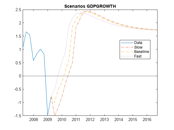
The extended forecasts cross paths in some cases. For example, for GDP, the speed-up of the economy after the crisis occurs sooner in the fast recovery scenario, and then it starts settling down towards a long-term mean level while the economy is just speeding up for other scenarios.
The macroeconomic scenarios are defined. This example proceeds to the credit analysis, specifically, the computation of expected credit losses (ECL).
Part 2: ECL Calculations
The second part of this example focuses on the workflow for computing the lifetime expected credit loss (ECL). ECL is the amount of provisions required for loan losses.
Part 2 works with an existing portfolio of loans for which there are three existing credit models: a lifetime probability of default (PD) model, a loss given default (LGD) model, and an exposure at default (EAD) model. These models predict lifetime PD, LGD, and EAD values several periods ahead, given projections on loan-specific predictor variables and the macroeconomic scenarios produced in Part 1.
Given the marginal PD, LGD, and EAD projections for different scenarios, you can use the portfolioECL (Risk Management Toolbox) function to estimate the lifetime loan loss provisions. This example presents a comparison of 1-year ECL vs. lifetime ECL and this corresponds to stage 1 vs. stage 2 of the IFRS 9 regulation. In this example, the estimated provisions for the lifetime ECL and 1-year ECL are very high because the three macroeconomic scenarios correspond to challenging economic conditions. For reference, this example also estimates 1-year provisions using an average macroeconomic scenario. This approach is similar to a through-the-cycle (TTC) method that shows in normal times the same models produce significantly lower provisions. You can use a visualization of credit projections and provisions for each ID to drill down to a loan level.
Part 2 describes the following workflow:
Both the portfolio data and the models are simulated to capture characteristics that may be found in practice and are intended only for illustration purposes.
Prepare for Loan Data for Macroeconomic Scenarios
The ECLPortfolioMacroExample.mat file contains loan portfolio data. This data is a simulated existing portfolio of loans. The ECLPortfolioSnapshot table indicates which loans are in the portfolio.
load ECLPortfolioMacroExample.mat

head(ECLPortfolioSnapshot,5)
ID Time Age ScoreGroupOrig Balance Limit EffIntRate
__ ___________ ___ ______________ _______ _____ __________
1 31-Mar-2009 12 LowRisk 3474 9000 5.04
2 31-Mar-2009 5 LowRisk 6232.7 9100 1.51
3 31-Mar-2009 3 HighRisk 2420.6 6000 3.13
4 31-Mar-2009 2 LowRisk 7274.2 10100 0.28
5 31-Mar-2009 1 MediumRisk 3611.8 5800 0.96
The ECLPortfolioProjections table contains portfolio projections. These values are projected for the remaining life of each loan and for each of the loan variables. For example, the age (measured in quarters) is required for the lifetime PD and LGD models. Because the first loan is 12 quarters old, the projected age for the remaining periods starts at 13 and goes up by one all the way to the end of the loan, at 20 quarters (5 years). All models use the score group at origination and that is a constant value. The loan-to-value (LTV) ratio included in this simulated data set and models is the LTV at origination, which is constant. In practice, if the most recent LTV were included, it would have to be projected all the way through the end of the life of each loan.
head(ECLPortfolioProjections,10)
    ID    Age    ScoreGroupOrig    LTVOrig    Limit       Time
    __    ___    ______________    _______    _____    ___________

    1     13        LowRisk        0.81866    9000     30-Jun-2009
    1     14        LowRisk        0.81866    9000     30-Sep-2009
    1     15        LowRisk        0.81866    9000     31-Dec-2009
    1     16        LowRisk        0.81866    9000     31-Mar-2010
    1     17        LowRisk        0.81866    9000     30-Jun-2010
    1     18        LowRisk        0.81866    9000     30-Sep-2010
    1     19        LowRisk        0.81866    9000     31-Dec-2010
    1     20        LowRisk        0.81866    9000     31-Mar-2011
    2      6        LowRisk        0.79881    9100     30-Jun-2009
    2      7        LowRisk        0.79881    9100     30-Sep-2009
The credit models need projected values of GDP growth, unemployment rate, and interest rate, all lagged by one period. First, store the macroeconomic information in the MacroScenarios table, where the macroeconomic scenarios are stacked.
ScenarioIDs = ["SlowRecovery";"Baseline";"FastRecovery"];
NumScenarios = length(ScenarioIDs);

MacroScenarios = table;
NumForecastPeriods = height(TTForecast)-1; % Remove initial period, keep future periods only
MacroScenarios.ScenarioID = repelem(ScenarioIDs,NumForecastPeriods);
MacroScenarios.Time = repmat(TTForecast.Time(2:end),NumScenarios,1);

MacroScenarios.GDPGROWTHLAG = NaN(height(MacroScenarios),1);
MacroScenarios.GDPGROWTHLAG(MacroScenarios.ScenarioID=="SlowRecovery") = TTSlow.GDPGROWTH(1:end-1);
MacroScenarios.GDPGROWTHLAG(MacroScenarios.ScenarioID=="Baseline") = TTBaseline.GDPGROWTH(1:end-1);
MacroScenarios.GDPGROWTHLAG(MacroScenarios.ScenarioID=="FastRecovery") = TTFast.GDPGROWTH(1:end-1);

MacroScenarios.UNRATELAG = NaN(height(MacroScenarios),1);
MacroScenarios.UNRATELAG(MacroScenarios.ScenarioID=="SlowRecovery") = TTSlow.UNRATE(1:end-1);
MacroScenarios.UNRATELAG(MacroScenarios.ScenarioID=="Baseline") = TTBaseline.UNRATE(1:end-1);
MacroScenarios.UNRATELAG(MacroScenarios.ScenarioID=="FastRecovery") = TTFast.UNRATE(1:end-1);

MacroScenarios.TB3MSLAG = NaN(height(MacroScenarios),1);
MacroScenarios.TB3MSLAG(MacroScenarios.ScenarioID=="SlowRecovery") = TTSlow.TB3MS(1:end-1);
MacroScenarios.TB3MSLAG(MacroScenarios.ScenarioID=="Baseline") = TTBaseline.TB3MS(1:end-1);
MacroScenarios.TB3MSLAG(MacroScenarios.ScenarioID=="FastRecovery") = TTFast.TB3MS(1:end-1);

head(MacroScenarios)
      ScenarioID         Time        GDPGROWTHLAG    UNRATELAG    TB3MSLAG
    ______________    ___________    ____________    _________    ________

    "SlowRecovery"    30-Jun-2009      -0.78191          8.5          0.21
    "SlowRecovery"    30-Sep-2009          -1.5          9.3          -0.5
    "SlowRecovery"    31-Dec-2009          -1.2         10.1         -0.25
    "SlowRecovery"    31-Mar-2010          -0.8           11         -0.15
    "SlowRecovery"    30-Jun-2010          -0.3         10.5         -0.05
    "SlowRecovery"    30-Sep-2010           0.1          9.9             0
    "SlowRecovery"    31-Dec-2010           0.5          9.1          0.05
    "SlowRecovery"    31-Mar-2011        1.8334       8.6536      -0.19292
To make predictions with the credit models, use the macroeconomic scenarios together with the loan data containing all the loan projection periods correctly aligned in time with the macroeconomic projected values. There are different ways to implement this. In this example, you can stack the portfolio projections three times, one for each scenario, and then join the stacked projections with the macro scenarios. Although this stacking method uses more memory, you can easily drill down to the loan level for different scenarios (see Loan-Level Results).
Stack portfolio projections by scenario in the ECLProjectionsByScenario table, and apply a join operation with the MacroScenarios table. The result is to add the macro variables to the larger table, using the Time and ScenarioID variables as keys for the join.
ECLProjectionsByScenario = repmat(ECLPortfolioProjections,NumScenarios,1);
ECLProjectionsByScenario = addvars(ECLProjectionsByScenario,repelem(ScenarioIDs,height(ECLPortfolioProjections)),'Before','ID','NewVariableName','ScenarioID');
ECLProjectionsByScenario = join(ECLProjectionsByScenario,MacroScenarios);
head(ECLProjectionsByScenario,10)
      ScenarioID      ID    Age    ScoreGroupOrig    LTVOrig    Limit       Time        GDPGROWTHLAG    UNRATELAG    TB3MSLAG
    ______________    __    ___    ______________    _______    _____    ___________    ____________    _________    ________

    "SlowRecovery"    1     13        LowRisk        0.81866    9000     30-Jun-2009      -0.78191          8.5          0.21
    "SlowRecovery"    1     14        LowRisk        0.81866    9000     30-Sep-2009          -1.5          9.3          -0.5
    "SlowRecovery"    1     15        LowRisk        0.81866    9000     31-Dec-2009          -1.2         10.1         -0.25
    "SlowRecovery"    1     16        LowRisk        0.81866    9000     31-Mar-2010          -0.8           11         -0.15
    "SlowRecovery"    1     17        LowRisk        0.81866    9000     30-Jun-2010          -0.3         10.5         -0.05
    "SlowRecovery"    1     18        LowRisk        0.81866    9000     30-Sep-2010           0.1          9.9             0
    "SlowRecovery"    1     19        LowRisk        0.81866    9000     31-Dec-2010           0.5          9.1          0.05
    "SlowRecovery"    1     20        LowRisk        0.81866    9000     31-Mar-2011        1.8334       8.6536      -0.19292
    "SlowRecovery"    2      6        LowRisk        0.79881    9100     30-Jun-2009      -0.78191          8.5          0.21
    "SlowRecovery"    2      7        LowRisk        0.79881    9100     30-Sep-2009          -1.5          9.3          -0.5
Predict Lifetime PD, LGD, and EAD
Load the existing credit models and use them to make predictions using the prepared data. In this workflow, new credit models for PD, LGD, and EAD are not fit; the assumption is that these credit models were previously fit and reviewed and are ready to use for ECL calculations. The credit models are all instances of models created with Risk Management Toolbox™ using fitLifetimePDModel (Risk Management Toolbox), fitLGDModel (Risk Management Toolbox), and fitEADModel (Risk Management Toolbox).
load ECLCreditModelsMacroExample.matThe lifetime PD model is a Probit (Risk Management Toolbox) model with the predictors: age of the loan, score group at origination, LTV ratio at origination, and the lagged GDP growth and unemployment rate values.
disp(pdECLModel)
  Probit with properties:

            ModelID: "PD-ECL-Probit"
        Description: "Lifetime PD model example fitted to simulated data."
    UnderlyingModel: [1×1 classreg.regr.CompactGeneralizedLinearModel]
              IDVar: "ID"
             AgeVar: "Age"
           LoanVars: ["ScoreGroupOrig"    "LTVOrig"]
          MacroVars: ["GDPGROWTHLAG"    "UNRATELAG"]
        ResponseVar: "Default"
         WeightsVar: ""
       TimeInterval: []
The LGD model is a Tobit (Risk Management Toolbox) model with the predictors: age of the loan, score group at origination, LTV ratio at origination, and the lagged GDP growth.
disp(lgdECLModel)
  Tobit with properties:

      CensoringSide: "both"
          LeftLimit: 0
         RightLimit: 1
            Weights: [0×1 double]
            ModelID: "LGD-ECL-Tobit"
        Description: "LGD model example fitted to simulated data."
    UnderlyingModel: [1×1 risk.internal.credit.TobitModel]
      PredictorVars: ["Age"    "ScoreGroupOrig"    "LTVOrig"    "GDPGROWTHLAG"]
        ResponseVar: "LGD"
         WeightsVar: ""
The EAD model is a Regression (Risk Management Toolbox) model, based on the limit conversion factor (LCF) conversion measure, with the predictors: score group at origination, LTV ratio at origination, and the lagged unemployment rate and interest rate values. Because the underlying model predicts LCF, the EAD model requires the credit limit variable to make EAD predictions, even though the credit limit is not a predictor of the underlying LCF model.
disp(eadECLModel)
  Regression with properties:

    ConversionTransform: "logit"
      BoundaryTolerance: 1.0000e-07
                ModelID: "EAD-ECL-Regression"
            Description: "EAD model example fitted to simulated data."
        UnderlyingModel: [1×1 classreg.regr.CompactLinearModel]
          PredictorVars: ["ScoreGroupOrig"    "LTVOrig"    "UNRATELAG"    "TB3MSLAG"]
            ResponseVar: "EAD"
               LimitVar: "Limit"
               DrawnVar: ""
      ConversionMeasure: "lcf"
Store the predictions in the ECLProjectionsByScenario table. The predictions can also be stored in separate tables and used directly as inputs for the portfolioECL (Risk Management Toolbox) function. For an example of using separate tables, see Calculate ECL Based on Marginal PD, LGD, and EAD Predictions (Risk Management Toolbox). Storing predictions in the ECLProjectionsByScenario table with scenarios stacked allows you to review prediction details at a very granular level because the predictions are stored side by side with projected predictor values in each row.
Store the lifetime (cumulative) PD and the marginal PD. Typically, the cumulative PD is used for reporting purposes and the marginal PD is used as an input for ECL computations with the portfolioECL (Risk Management Toolbox) function.
ECLProjectionsByScenario.PDLifetime = zeros(height(ECLProjectionsByScenario),1);
ECLProjectionsByScenario.PDMarginal = zeros(height(ECLProjectionsByScenario),1);
ECLProjectionsByScenario.LGD = zeros(height(ECLProjectionsByScenario),1);
ECLProjectionsByScenario.EAD = zeros(height(ECLProjectionsByScenario),1);

for ii=1:NumScenarios

   ScenIndECLData = ECLProjectionsByScenario.ScenarioID==ScenarioIDs(ii);

   ECLProjectionsByScenario.PDLifetime(ScenIndECLData) = predictLifetime(pdECLModel,ECLProjectionsByScenario(ScenIndECLData,:)); % cumulative
   ECLProjectionsByScenario.PDMarginal(ScenIndECLData) = predictLifetime(pdECLModel,ECLProjectionsByScenario(ScenIndECLData,:),ProbabilityType="marginal");
   ECLProjectionsByScenario.LGD(ScenIndECLData) = predict(lgdECLModel,ECLProjectionsByScenario(ScenIndECLData,:));
   ECLProjectionsByScenario.EAD(ScenIndECLData) = predict(eadECLModel,ECLProjectionsByScenario(ScenIndECLData,:));

end
head(ECLProjectionsByScenario,10)
      ScenarioID      ID    Age    ScoreGroupOrig    LTVOrig    Limit       Time        GDPGROWTHLAG    UNRATELAG    TB3MSLAG    PDLifetime    PDMarginal      LGD       EAD
    ______________    __    ___    ______________    _______    _____    ___________    ____________    _________    ________    __________    __________    _______    ______

    "SlowRecovery"    1     13        LowRisk        0.81866    9000     30-Jun-2009      -0.78191          8.5          0.21    0.0092969     0.0092969     0.29862    4730.2
    "SlowRecovery"    1     14        LowRisk        0.81866    9000     30-Sep-2009          -1.5          9.3          -0.5     0.020034      0.010737     0.33245    5111.1
    "SlowRecovery"    1     15        LowRisk        0.81866    9000     31-Dec-2009          -1.2         10.1         -0.25     0.030184       0.01015     0.31095      6185
    "SlowRecovery"    1     16        LowRisk        0.81866    9000     31-Mar-2010          -0.8           11         -0.15     0.039815     0.0096304     0.28469    7073.3
    "SlowRecovery"    1     17        LowRisk        0.81866    9000     30-Jun-2010          -0.3         10.5         -0.05     0.046246     0.0064312      0.2543      6703
    "SlowRecovery"    1     18        LowRisk        0.81866    9000     30-Sep-2010           0.1          9.9             0     0.050458     0.0042121     0.23014    6152.4
    "SlowRecovery"    1     19        LowRisk        0.81866    9000     31-Dec-2010           0.5          9.1          0.05      0.05303     0.0025718     0.20708    5309.3
    "SlowRecovery"    1     20        LowRisk        0.81866    9000     31-Mar-2011        1.8334       8.6536      -0.19292     0.054387     0.0013569     0.14745    4589.9
    "SlowRecovery"    2      6        LowRisk        0.79881    9100     30-Jun-2009      -0.78191          8.5          0.21      0.02793       0.02793      0.3326    4763.5
    "SlowRecovery"    2      7        LowRisk        0.79881    9100     30-Sep-2009          -1.5          9.3          -0.5     0.058871      0.030942     0.36752    5148.9
Compute Lifetime ECL
Compute the lifetime ECL using the portfolioECL (Risk Management Toolbox) function. The inputs to this function are tables, where the first column is an ID variable that indicates which rows correspond to which loan. Because the projections cover multiple periods for each loan, and the remaining life of different loans may be different, the ID variable is an important input. Then, for each ID, the credit projections must be provided, period by period, until the end of the life of each loan. Typically, the marginal PD has a multi-period and multi-scenario size. However, in some situations, more commonly for LGD or EAD inputs, the credit projections may not have values for each period, or may not be sensitive to the scenarios. A typical case for this situation is a loan that repays the principal at maturity, where the exposure is considered constant for each period and independent of the macroeconomic scenarios. In this case, the EAD table input has one scalar value per ID that applies for all periods and all scenarios. To offer flexibility for different input dimensions for marginal PD, LGD, and EAD inputs, these inputs are separated into three separate tables in the syntax of portfolioECL (Risk Management Toolbox).
Reformat the credit projections stored in the ECLProjectionsByScenario table into an intermediate table that includes the Time variable. You can use these intermediate tables to look at the detailed predictions period-by-period with different scenarios side-by-side. Also, these tables with a Time variable are useful for logical indexing to extract the predictions for only the first year.
PDMarginalUnstacked = ECLProjectionsByScenario(:,["ScenarioID" "ID" "Time" "PDMarginal"]);
PDMarginalUnstacked = unstack(PDMarginalUnstacked,"PDMarginal","ScenarioID");
PDMarginalUnstacked = movevars(PDMarginalUnstacked,"SlowRecovery","Before","Baseline");
disp(head(PDMarginalUnstacked))
    ID       Time        SlowRecovery    Baseline     FastRecovery
    __    ___________    ____________    _________    ____________

    1     30-Jun-2009     0.0092969      0.0092969      0.0092969
    1     30-Sep-2009      0.010737      0.0090867      0.0078466
    1     31-Dec-2009       0.01015      0.0076948       0.005958
    1     31-Mar-2010     0.0096304       0.006847      0.0045918
    1     30-Jun-2010     0.0064312      0.0045587      0.0032064
    1     30-Sep-2010     0.0042121      0.0030213      0.0019542
    1     31-Dec-2010     0.0025718      0.0016771      0.0013505
    1     31-Mar-2011     0.0013569      0.0011649     0.00096951
LGDUnstacked = ECLProjectionsByScenario(:,["ScenarioID" "ID" "Time" "LGD"]);
LGDUnstacked = unstack(LGDUnstacked,"LGD","ScenarioID");
LGDUnstacked = movevars(LGDUnstacked,"SlowRecovery","Before","Baseline");

EADUnstacked = ECLProjectionsByScenario(:,["ScenarioID" "ID" "Time" "EAD"]);
EADUnstacked = unstack(EADUnstacked,"EAD","ScenarioID");
EADUnstacked = movevars(EADUnstacked,"SlowRecovery","Before","Baseline");
The final step to preparing the inputs for portfolioECL (Risk Management Toolbox) is to remove the Time column. There are other ways to prepare these inputs, for example, you can store the columns side-by-side directly during prediction. In this example, the extra steps for preparation are illustrated so that you can use the ECLProjectionsByScenario table for detailed analysis at a loan level (see Loan-Level Results).
PDMarginalLifetimeInput = PDMarginalUnstacked(:,[1 3:end]);
disp(head(PDMarginalLifetimeInput))
    ID    SlowRecovery    Baseline     FastRecovery
    __    ____________    _________    ____________

    1      0.0092969      0.0092969      0.0092969
    1       0.010737      0.0090867      0.0078466
    1        0.01015      0.0076948       0.005958
    1      0.0096304       0.006847      0.0045918
    1      0.0064312      0.0045587      0.0032064
    1      0.0042121      0.0030213      0.0019542
    1      0.0025718      0.0016771      0.0013505
    1      0.0013569      0.0011649     0.00096951
LGDLifetimeInput = LGDUnstacked(:,[1 3:end]);
EADLifetimeInput = EADUnstacked(:,[1 3:end]);
Each loan has an effective interest rate for discounting that is determined at loan recognition.
EIRInput = ECLPortfolioSnapshot(:,["ID" "EffIntRate"]);
EIRInput.EffIntRate = EIRInput.EffIntRate/100; % Convert to decimal
Use the portfolioECL (Risk Management Toolbox) function.
[totalECL,idECL,periodECL] = portfolioECL(PDMarginalLifetimeInput,LGDLifetimeInput,EADLifetimeInput,...
   ScenarioNames=ScenarioIDs,ScenarioProbabilities=scenarioProb,InterestRate=EIRInput);
The totalECL output is the lifetime ECL of the portfolio which is the total provisions amount required by the portfolio.
fprintf('Total Portfolio Lifetime ECL: %s',cur2str(totalECL))Total Portfolio Lifetime ECL: $67701.21
The idECL output is the lifetime ECL at a loan level. Join the idECL output with the score group and the balance information from the ECL portfolio snapshot table. With this data, you can compute the lifetime ECL as a percent of the loan balance. You can also aggregate by score group. The TotalsByScore table shows that the lifetime ECL is significantly higher for lower quality score groups.
idECL = join(idECL,ECLPortfolioSnapshot(:,["ID" "ScoreGroupOrig" "Balance"]));
idECL.ECLPercent = 100*idECL.ECL./idECL.Balance;
TotalsByScore = groupsummary(idECL,"ScoreGroupOrig","sum",["ECL" "Balance"]);
TotalsByScore.ECLPercent = 100*TotalsByScore.sum_ECL./TotalsByScore.sum_Balance
TotalsByScore=3×5 table
    ScoreGroupOrig    GroupCount    sum_ECL    sum_Balance    ECLPercent
    ______________    __________    _______    ___________    __________

      HighRisk            76         22027      1.828e+05        12.05
      MediumRisk         121         23921      3.312e+05       7.2225
      LowRisk            130         21753     5.9629e+05       3.6481
The provisions in TotalsByScore table are very high. These results are explored in the Compute 1-Year ECL and Compute 1-Year ECL with Average Macroeconomic Levels sections.
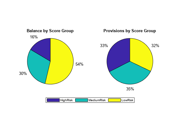
Visualize the distribution of the portfolio balance and the distribution of provisions by score group. Only about 1/6 of the assets are allocated to high-risk loans, yet the provisions for high risk make up about 1/3 of the total provisions. On the other end, more than half of the assets are allocated to low-risk loans, yet the provisions for low risk are less than 1/3 of the total provisions.
figure
tiledlayout(1,2)
nexttile
pie(TotalsByScore.sum_Balance)
title('Balance by Score Group')
nexttile
pie(TotalsByScore.sum_ECL)
title('Provisions by Score Group')
leg = legend(TotalsByScore.ScoreGroupOrig,'Location','south','Orientation','horizontal');
leg.Layout.Tile = 'south';
Compute 1-Year ECL
As noted in Compute Lifetime ECL, the lifetime provisions in TotalsByScore table are very high. To better understand why, you can compute 1-year provisions to understand the impact of the lifetime part of the ECL beyond the first year.
The difference between lifetime ECL and 1-year ECL is important for the IFRS 9 regulation where stage 1 loans (performing loans) use 1-year ECL for provisioning, whereas stage 2 loans (increased credit risk) and stage 3 loans (credit impaired) use lifetime ECL. [1]
To obtain a 1-year ECL, prepare the marginal PD, LGD, and EAD input tables so that they cover one year ahead. You can leverage the unstacked tables created in Compute Lifetime ECL. These unstacked tables contain a Time variable to do logical indexing and obtain the inputs for a 1-year ECL. In the new inputs, each ID has only four periods and any loan with a remaining life of less than four quarters has fewer periods.
FourthQuarterAhead = ECLPortfolioProjections.Time(4);
PDMarginal1YearInput = PDMarginalUnstacked(PDMarginalUnstacked.Time<=FourthQuarterAhead,[1 3:end]);
disp(head(PDMarginal1YearInput))
    ID    SlowRecovery    Baseline     FastRecovery
    __    ____________    _________    ____________

    1      0.0092969      0.0092969     0.0092969
    1       0.010737      0.0090867     0.0078466
    1        0.01015      0.0076948      0.005958
    1      0.0096304       0.006847     0.0045918
    2        0.02793        0.02793       0.02793
    2       0.030942       0.026838      0.023675
    2       0.028822       0.022818      0.018364
    2       0.026954       0.020285      0.014466
LGD1YearInput = LGDUnstacked(LGDUnstacked.Time<=FourthQuarterAhead,[1 3:end]);
EAD1YearInput = EADUnstacked(EADUnstacked.Time<=FourthQuarterAhead,[1 3:end]);
Use portfolioECL (Risk Management Toolbox) with the new inputs.
[totalECL1Year,idECL1Year,periodECL1Year] = portfolioECL(PDMarginal1YearInput,LGD1YearInput,EAD1YearInput,...
   ScenarioNames=ScenarioIDs,ScenarioProbabilities=scenarioProb,InterestRate=EIRInput);
Expand the ID level ECL table with the score group and balance information.
idECL1Year.ScoreGroupOrig = idECL.ScoreGroupOrig;
idECL1Year.Balance = idECL.Balance;
idECL1Year.ECLPercent = 100*idECL1Year.ECL./idECL1Year.Balance;

TotalsByScore1Year = groupsummary(idECL1Year,"ScoreGroupOrig","sum",["ECL" "Balance"]);
TotalsByScore1Year.ECLPercent = 100*TotalsByScore1Year.sum_ECL./TotalsByScore1Year.sum_Balance;
Compare the 1-year ECL with the lifetime ECL by plotting the lifetime and 1-year ECL values as a proportion of balance for each score group.
figure;
bar([TotalsByScore.ECLPercent TotalsByScore1Year.ECLPercent])
xticklabels(TotalsByScore.ScoreGroupOrig)
ylabel('ECL as % of Balance')
legend('Lifetime ECL','1-Year ECL')
title('ECL, Lifetime vs. 1 Year')
grid on
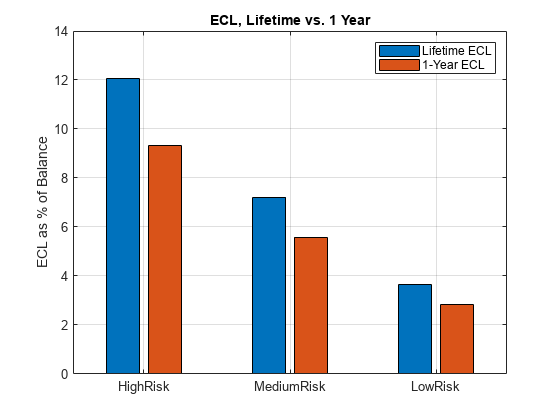
The lifetime ECL shows an important increase with respect to the 1-year ECL. However, the 1-year ECL values are high. In general, the increment from 1-year ECL to lifetime ECL is not expected to be large because marginal PD values tend to decrease as loans age, and in some cases, the risk implied by LGD and EAD projections can also decrease with time. An example of this behavior is an amortizing loan.
The macroeconomic scenarios in this example are extremely adverse and the provisions are conditional on the macroeconomic scenarios. Compute 1-Year ECL with Average Macroeconomic Levels explores the impact of these adverse scenarios on the ECL estimates.
Compute 1-Year ECL with Average Macroeconomic Levels
To compare the 1-year ECL with more normal macroeconomic conditions, the macroeconomic scenarios from Define Macroeconomic Scenarios are replaced with a long-term average of the macroeconomic variables. To simplify, use the long-term average of the macroeconomic variables to make predictions only four quarters ahead. This approach is similar to a through-the-cycle (TTC) reserving approach because the credit projections reflect average macroeconomic conditions.
Use the mean macroeconomic levels over the entire sample.
MeanGDPGROWTH = mean(DataMacro.GDPGROWTH);
MeanUNRATE = mean(DataMacro.UNRATE);
MeanTB3MS = mean(DataMacro.TB3MS);
To make predictions, you need the projected predictors values and data only one year ahead.
ECLPortfolio1YearMacroAverage = ECLPortfolioProjections(ECLPortfolioProjections.Time<=FourthQuarterAhead,:);
ECLPortfolio1YearMacroAverage.GDPGROWTHLAG = zeros(height(ECLPortfolio1YearMacroAverage),1);
ECLPortfolio1YearMacroAverage.UNRATELAG = zeros(height(ECLPortfolio1YearMacroAverage),1);
ECLPortfolio1YearMacroAverage.TB3MSLAG = zeros(height(ECLPortfolio1YearMacroAverage),1);
Append the macroeconomic average values and use the same average value for all periods going forward.
ECLPortfolio1YearMacroAverage.GDPGROWTHLAG(:) = MeanGDPGROWTH;
ECLPortfolio1YearMacroAverage.UNRATELAG(:) = MeanUNRATE;
ECLPortfolio1YearMacroAverage.TB3MSLAG(:) = MeanTB3MS;
Predict credit values. You need only the marginal PD values for ECL calculations, but you can also store the lifetime PD values for the analysis in the Loan-Level Results section.
ECLPortfolio1YearMacroAverage.PDLifetime = predictLifetime(pdECLModel,ECLPortfolio1YearMacroAverage);
ECLPortfolio1YearMacroAverage.PDMarginal = predictLifetime(pdECLModel,ECLPortfolio1YearMacroAverage,ProbabilityType="marginal");
ECLPortfolio1YearMacroAverage.LGD = predict(lgdECLModel,ECLPortfolio1YearMacroAverage);
ECLPortfolio1YearMacroAverage.EAD = predict(eadECLModel,ECLPortfolio1YearMacroAverage);
In this case, the inputs for the portfolioECL (Risk Management Toolbox) function have only one scenario.
PDMarginal1YearMacroAverageInput = ECLPortfolio1YearMacroAverage(:,["ID" "PDMarginal"]);
LGD1YearMacroAverageInput = ECLPortfolio1YearMacroAverage(:,["ID" "LGD"]);
EAD1YearMacroAverageInput = ECLPortfolio1YearMacroAverage(:,["ID" "EAD"]);
Obtain the 1-year ECL and expand the loan-level results table.
[totalECL1YearMacroAverage,idECL1YearMacroAverage,periodECL1YearMacroAverage] = portfolioECL(PDMarginal1YearMacroAverageInput,LGD1YearMacroAverageInput,EAD1YearMacroAverageInput,InterestRate=EIRInput);

idECL1YearMacroAverage.ScoreGroupOrig = idECL.ScoreGroupOrig;
idECL1YearMacroAverage.Balance = idECL.Balance;
idECL1YearMacroAverage.ECLPercent = 100*idECL1YearMacroAverage.ECL./idECL1YearMacroAverage.Balance;

TotalsByScore1YearMacroAverage = groupsummary(idECL1YearMacroAverage,"ScoreGroupOrig","sum",["ECL" "Balance"]);
TotalsByScore1YearMacroAverage.ECLPercent = 100*TotalsByScore1YearMacroAverage.sum_ECL./TotalsByScore1YearMacroAverage.sum_Balance;
Compare the 1-year ECL with average macroeconomic values to the 1-year ECL and lifetime ECL approach using the initial macroeconomic scenarios.
figure;
bar([TotalsByScore.ECLPercent TotalsByScore1Year.ECLPercent TotalsByScore1YearMacroAverage.ECLPercent])
xticklabels(TotalsByScore.ScoreGroupOrig)
ylabel('ECL as % of Balance')
legend('Lifetime ECL','1-Year ECL','1-Year ECL, Macro Average')
title('ECL, Lifetime vs. 1 Year vs. 1 Year Macro Average')
grid on
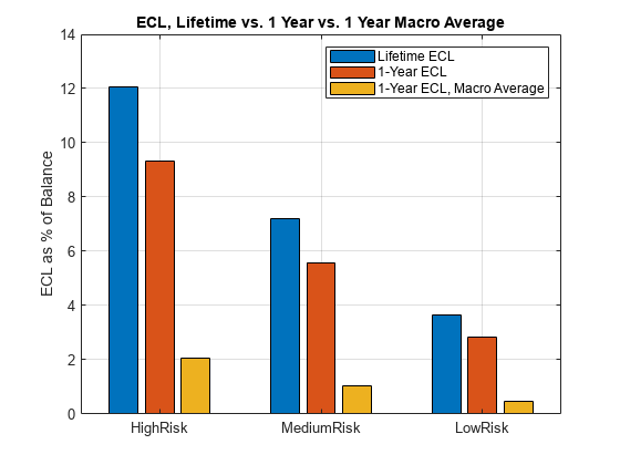
These results show that the severely adverse macroeconomic scenarios defined in Define Macroeconomic Scenarios drive the high provisions. The 1-year ECL values with average macroeconomic levels are much lower with the low-risk 1-year ECL at 0.5% of the current provisions balance. The medium-risk 1-year ECL is at 1% of the current provisions balance and the high-risk 1-year ECL is 2% of the current provisions balance.
Visualize Loan-Level Results
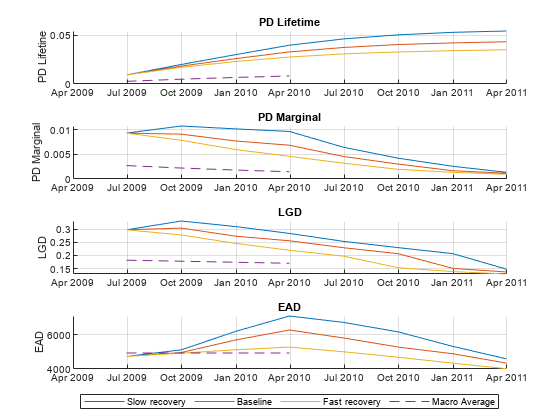
You can explore the ECL predictions and the results at a loan level. Use SelectedID to enter any loan ID in the portfolio. The resulting visualizations show the predicted lifetime PD, marginal PD, LGD, and EAD over the remaining life of the loan. The plot shows the predictions for each macroeconomic scenario defined in Define Macroeconomic Scenarios as well as the macroeconomic average scenario (1-year predictions only).
SelectedID =1; IDDataLifetime = ECLProjectionsByScenario(ECLProjectionsByScenario.ID==SelectedID,:); IDData1YearMacroAverage = ECLPortfolio1YearMacroAverage(ECLPortfolio1YearMacroAverage.ID==SelectedID,:); figure; t = tiledlayout(4,1); nexttile hold on for ii=1:NumScenarios ScenPlotInd = IDDataLifetime.ScenarioID==ScenarioIDs(ii); plot(IDDataLifetime.Time(ScenPlotInd),IDDataLifetime.PDLifetime(ScenPlotInd)) end plot(IDData1YearMacroAverage.Time,IDData1YearMacroAverage.PDLifetime,'--') hold off ylabel('PD Lifetine') title('PD Lifetime') grid on nexttile hold on for ii=1:NumScenarios ScenPlotInd = IDDataLifetime.ScenarioID==ScenarioIDs(ii); plot(IDDataLifetime.Time(ScenPlotInd),IDDataLifetime.PDMarginal(ScenPlotInd)) end plot(IDData1YearMacroAverage.Time,IDData1YearMacroAverage.PDMarginal,'--') hold off ylabel('PD Marginal') title('PD Marginal') grid on nexttile hold on for ii=1:NumScenarios ScenPlotInd = IDDataLifetime.ScenarioID==ScenarioIDs(ii); plot(IDDataLifetime.Time(ScenPlotInd),IDDataLifetime.LGD(ScenPlotInd)) end plot(IDData1YearMacroAverage.Time,IDData1YearMacroAverage.LGD,'--') hold off ylabel('LGD') title('LGD') grid on nexttile hold on for ii=1:NumScenarios ScenPlotInd = IDDataLifetime.ScenarioID==ScenarioIDs(ii); plot(IDDataLifetime.Time(ScenPlotInd),IDDataLifetime.EAD(ScenPlotInd)) end plot(IDData1YearMacroAverage.Time,IDData1YearMacroAverage.EAD,'--') hold off ylabel('EAD') title('EAD') grid on leg = legend("Slow recovery","Baseline","Fast recovery","Macro Average","Orientation","horizontal"); leg.Layout.Tile = 'south';
The following plot shows the ECL for the loan, the ECL for the lifetime case, the 1-year ECL case, and the 1-year ECL using average macroeconomic values.
figure;
IDECLInd = idECL.ID == SelectedID;
bar(categorical("Provisions"),[idECL.ECLPercent(IDECLInd) idECL1Year.ECLPercent(IDECLInd) idECL1YearMacroAverage.ECLPercent(IDECLInd)])
legend('Lifetime','1 Year','1 Year Macro Average')
ylabel('ECL as % of Balance')
TitleStr = sprintf('ID: %g, Score Group: %s',SelectedID,idECL.ScoreGroupOrig(IDECLInd));
title(TitleStr)
grid on

Conclusion
This example covers an entire workflow, including the determination of macroeconomic scenarios and the estimation of provisions using lifetime ECL computations. The example also shows some tools and visualizations to analyze the results at a portfolio level, score-group level, and loan level.
The example demonstrates tools from the Econometrics Toolbox™ and Risk Management Toolbox™ that support this workflow, including macroeconomic modeling tools such as vector autoregressive (VAR) models, and credit risk tools such as the lifetime probability of default (PD) models (fitLifetimePDModel (Risk Management Toolbox)), loss given default (LGD) models (fitLGDModel (Risk Management Toolbox)), exposure at default (EAD) models (fitEADModel (Risk Management Toolbox)), and the portfolioECL (Risk Management Toolbox) function.
References
[1] Bellini, Tiziano. IFRS 9 and CECL Credit Risk Modelling and Validation: A Practical Guide with Examples Worked in R and SAS. Elsevier, 2019.
[2] Breeden, Joseph. Living with CECL: The Modeling Dictionary. Prescient Models LLC, 2018.
[3] Roesch, Daniel and Harald Scheule. Deep Credit Risk: Machine Learning with Python. Independently published, 2020.
See Also
Functions
fitLifetimePDModel(Risk Management Toolbox) |fitEADModel(Risk Management Toolbox) |fitLGDModel(Risk Management Toolbox) |portfolioECL(Risk Management Toolbox) |estimate|forecast
Objects
Topics
- Expected Credit Loss Computation (Risk Management Toolbox)
- Modeling Probabilities of Default with Cox Proportional Hazards (Risk Management Toolbox)
- Model the United States Economy