summary
Generate summary table of backtest results
Description
summaryTable = summary(backtester)runBacktest function.
Examples
The MATLAB® backtesting engine runs backtests of portfolio investment strategies over time series of asset price data. You can use summary to compare multiple strategies over the same market scenario. This example shows how to examine the results of a backtest with two strategies.
Load Data
Load one year of stock price data. For readability, this example uses a subset of the DJIA stocks.
% Read table of daily adjusted close prices for 2006 DJIA stocks
T = readtable('dowPortfolio.xlsx');

% Prune the table to include only the dates and selected stocks
timeColumn = "Dates";
assetSymbols = ["BA", "CAT", "DIS", "GE", "IBM", "MCD", "MSFT"];
T = T(:,[timeColumn assetSymbols]);

% Convert to timetable
pricesTT = table2timetable(T,'RowTimes','Dates');

% View the final asset price timetable
head(pricesTT)
       Dates        BA       CAT      DIS      GE       IBM      MCD     MSFT
    ___________    _____    _____    _____    _____    _____    _____    _____

    03-Jan-2006    68.63    55.86    24.18     33.6    80.13    32.72    26.19
    04-Jan-2006    69.34    57.29    23.77    33.56    80.03    33.01    26.32
    05-Jan-2006    68.53    57.29    24.19    33.47    80.56    33.05    26.34
    06-Jan-2006    67.57    58.43    24.52     33.7    82.96    33.25    26.26
    09-Jan-2006    67.01    59.49    24.78    33.61    81.76    33.88    26.21
    10-Jan-2006    67.33    59.25    25.09    33.43     82.1    33.91    26.35
    11-Jan-2006     68.3    59.28    25.33    33.66    82.19     34.5    26.63
    12-Jan-2006     67.9    60.13    25.41    33.25    81.61    33.96    26.48
The inverse variance strategy requires some price history to initialize, so you can allocate a portion of the data to use for setting initial weights. By doing this, you can "warm start" the backtest.
warmupRange = 1:20;
testRange = 21:height(pricesTT);
Create Strategies
Define an investment strategy by using the backtestStrategy function. This example builds two strategies:
Equal weighted
Inverse variance
This example does not provide details on how to build the strategies. For more information on creating strategies, see backtestStrategy. The strategy rebalance functions are implemented in the Rebalance Functions section.
% Create the strategies
ewInitialWeights = equalWeightFcn([],pricesTT(warmupRange,:));
ewStrategy = backtestStrategy("EqualWeighted",@equalWeightFcn, ...
    'RebalanceFrequency',20, ...
    'TransactionCosts',[0.0025 0.005], ...
    'LookbackWindow',0, ...
    'InitialWeights',ewInitialWeights)
ewStrategy =
  backtestStrategy with properties:

                      Name: "EqualWeighted"
              RebalanceFcn: @equalWeightFcn
        RebalanceFrequency: 20
          TransactionCosts: [0.0025 0.0050]
            LookbackWindow: 0
            InitialWeights: [0.1429 0.1429 0.1429 0.1429 0.1429 0.1429 0.1429]
             ManagementFee: 0
     ManagementFeeSchedule: 1y
            PerformanceFee: 0
    PerformanceFeeSchedule: 1y
         PerformanceHurdle: 0
                  UserData: [0×0 struct]
            EngineDataList: [0×0 string]
ivInitialWeights = inverseVarianceFcn([],pricesTT(warmupRange,:));
ivStrategy = backtestStrategy("InverseVariance",@inverseVarianceFcn, ...
    'RebalanceFrequency',20, ...
    'TransactionCosts',[0.0025 0.005], ...
    'InitialWeights',ivInitialWeights)
ivStrategy =
  backtestStrategy with properties:

                      Name: "InverseVariance"
              RebalanceFcn: @inverseVarianceFcn
        RebalanceFrequency: 20
          TransactionCosts: [0.0025 0.0050]
            LookbackWindow: [0 Inf]
            InitialWeights: [0.1401 0.0682 0.0795 0.2187 0.1900 0.1875 0.1160]
             ManagementFee: 0
     ManagementFeeSchedule: 1y
            PerformanceFee: 0
    PerformanceFeeSchedule: 1y
         PerformanceHurdle: 0
                  UserData: [0×0 struct]
            EngineDataList: [0×0 string]
% Aggregate the strategies into an array
strategies = [ewStrategy ivStrategy];
Run Backtest
Create a backtesting engine and run a backtest over a year of stock data. For more information on creating backtesting engines, see backtestEngine. The software initializes several properties of the backtestEngine object to empty. These read-only properties are populated by the engine after you run the backtest.
% Create the backtesting engine using the default settings
backtester = backtestEngine(strategies)
backtester =
backtestEngine with properties:
Strategies: [1×2 backtestStrategy]
RiskFreeRate: 0
CashBorrowRate: 0
RatesConvention: "Annualized"
Basis: 0
InitialPortfolioValue: 10000
DateAdjustment: "Previous"
PayExpensesFromCash: 0
NumAssets: []
Returns: []
Positions: []
Turnover: []
BuyCost: []
SellCost: []
TransactionCosts: []
Fees: []
Run the backtest using runBacktest.
% Run the backtest
backtester = runBacktest(backtester,pricesTT(testRange,:));
Examine Summary Results
The summary function uses the results of the backtest and returns a table of high-level results from the backtest.
s1 = summary(backtester)
s1=9×2 table
EqualWeighted InverseVariance
_____________ _______________
TotalReturn 0.17567 0.17155
SharpeRatio 0.097946 0.10213
Volatility 0.0074876 0.0069961
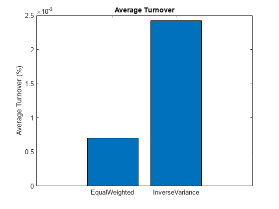
AverageTurnover 0.0007014 0.0024246
MaxTurnover 0.021107 0.097472
AverageReturn 0.00073178 0.00071296
MaxDrawdown 0.097647 0.096299
AverageBuyCost 0.018532 0.061913
AverageSellCost 0.037064 0.12383
Each row of the table output is a measurement of the performance of a strategy. Each strategy occupies a column. The summary function reports on the following metrics:
TotalReturn— The nonannulaized total return of the strategy, inclusive of fees, over the full backtest period.SharpeRatio— The nonannualized Sharpe ratio of each strategy over the backtest. For more information, seesharpe.Volatility— The nonannualized standard deviation of per-time-step strategy returns.AverageTurnover— The average per-time-step portfolio turnover, expressed as a decimal percentage.MaxTurnover— The maximum portfolio turnover in a single rebalance, expressed as a decimal percentage.AverageReturn—The arithmetic mean of the per-time step portfolio returns.MaxDrawdown— The maximum drawdown of the portfolio, expressed as a decimal percentage. For more information, seemaxdrawdown.AverageBuyCost— The average per-time-step transaction costs the portfolio incurred for asset purchases.AverageSellCost— The average per-time-step transaction costs the portfolio incurred for asset sales.
Sometimes it is useful to transpose the summary table when plotting the metrics of different strategies.
s2 = rows2vars(s1);
s2.Properties.VariableNames{1} = 'StrategyName's2=2×10 table
StrategyName TotalReturn SharpeRatio Volatility AverageTurnover MaxTurnover AverageReturn MaxDrawdown AverageBuyCost AverageSellCost
___________________ ___________ ___________ __________ _______________ ___________ _____________ ___________ ______________ _______________
{'EqualWeighted' } 0.17567 0.097946 0.0074876 0.0007014 0.021107 0.00073178 0.097647 0.018532 0.037064
{'InverseVariance'} 0.17155 0.10213 0.0069961 0.0024246 0.097472 0.00071296 0.096299 0.061913 0.12383
bar(s2.AverageTurnover)
title('Average Turnover')
ylabel('Average Turnover (%)')
set(gca,'xticklabel',s2.StrategyName)
Examine Detailed Results
After you run the backtest, the backtestEngine object updates the read-only fields with the detailed results of the backtest. The Returns, Positions, Turnover, BuyCost, SellCost, and Fees properties each contain a timetable of results. Since this example uses daily price data in the backtest, these timetables hold daily results.
backtester
backtester =
  backtestEngine with properties:

               Strategies: [1×2 backtestStrategy]
             RiskFreeRate: 0
           CashBorrowRate: 0
          RatesConvention: "Annualized"
                    Basis: 0
    InitialPortfolioValue: 10000
           DateAdjustment: "Previous"
      PayExpensesFromCash: 0
                NumAssets: 7
                  Returns: [230×2 timetable]
                Positions: [1×1 struct]
                 Turnover: [230×2 timetable]
                  BuyCost: [230×2 timetable]
                 SellCost: [230×2 timetable]
         TransactionCosts: [1×1 struct]
                     Fees: [1×1 struct]
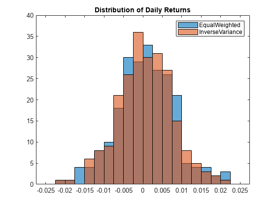
Returns
The Returns property holds a timetable of strategy (simple) returns for each time step. These returns are inclusive of all transaction fees.
head(backtester.Returns)
       Time        EqualWeighted    InverseVariance
    ___________    _____________    _______________

    02-Feb-2006      -0.007553        -0.0070957
    03-Feb-2006     -0.0037771         -0.003327
    06-Feb-2006     -0.0010094        -0.0014312
    07-Feb-2006      0.0053284         0.0020578
    08-Feb-2006      0.0099755         0.0095781
    09-Feb-2006     -0.0026871        -0.0014999
    10-Feb-2006      0.0048374         0.0059589
    13-Feb-2006     -0.0056868        -0.0051232
binedges = -0.025:0.0025:0.025;
h1 = histogram(backtester.Returns.EqualWeighted,'BinEdges',binedges);
hold on
histogram(backtester.Returns.InverseVariance,'BinEdges',binedges);
hold off
title('Distribution of Daily Returns')
legend([strategies.Name]);
Positions
The Positions property holds a structure of timetables, one per strategy.
backtester.Positions
ans = struct with fields:
      EqualWeighted: [231×8 timetable]
    InverseVariance: [231×8 timetable]
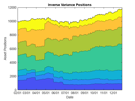
The Positions timetable of each strategy holds the per-time-step positions for each asset as well as the Cash asset (which earns the risk-free rate). The Positions timetables contain one more row than the other results timetables because the Positions timetables include initial positions of the strategy as their first row. You can consider the initial positions as the Time = 0 portfolio positions. In this example, the Positions timetables start with February 1, while the others start on February 2.
head(backtester.Positions.InverseVariance)
       Time           Cash          BA       CAT       DIS        GE       IBM       MCD       MSFT
    ___________    ___________    ______    ______    ______    ______    ______    ______    ______

    01-Feb-2006              0    1401.2    682.17    795.14    2186.8    1900.1    1874.9    1159.8
    02-Feb-2006              0    1402.8    673.74    789.74    2170.8    1883.5    1863.6      1145
    03-Feb-2006     1.0987e-12    1386.5     671.2     787.2    2167.3    1854.3    1890.5      1139
    06-Feb-2006     1.0971e-12    1391.9    676.78    785.62    2161.1    1843.6    1899.1    1123.8
    07-Feb-2006              0      1400    661.66    840.23    2131.9    1851.6    1902.3    1114.5
    08-Feb-2006    -2.2198e-12    1409.8     677.9    846.58    2160.4    1878.2      1911    1113.2
    09-Feb-2006              0    1414.8    674.35    840.87    2172.2      1869    1908.3    1102.6
    10-Feb-2006              0    1425.1    677.29     839.6    2195.8    1890.6    1909.3    1103.9
% Plot the change of asset allocation over time
t = backtester.Positions.InverseVariance.Time;
positions = backtester.Positions.InverseVariance.Variables;
h = area(t,positions);
title('Inverse Variance Positions');
xlabel('Date');
ylabel('Asset Positions');
xtickformat('MM/dd');
ylim([0 12000])
xlim([t(1) t(end)])
cm = parula(numel(h));
for i = 1:numel(h)
    set(h(i),'FaceColor',cm(i,:));
end
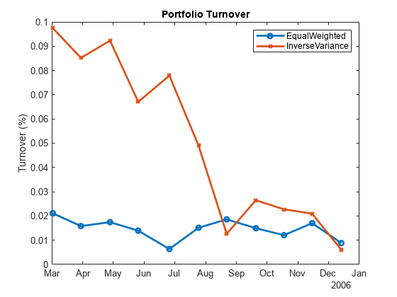
Turnover
The Turnover timetable holds the per-time-step portfolio turnover.
head(backtester.Turnover)
       Time        EqualWeighted    InverseVariance
    ___________    _____________    _______________

    02-Feb-2006          0                 0
    03-Feb-2006          0                 0
    06-Feb-2006          0                 0
    07-Feb-2006          0                 0
    08-Feb-2006          0                 0
    09-Feb-2006          0                 0
    10-Feb-2006          0                 0
    13-Feb-2006          0                 0
Depending on your rebalance frequency, the Turnover table can contain mostly zeros. Removing these zeros when you visualize the portfolio turnover is useful.
nonZeroIdx = sum(backtester.Turnover.Variables,2) > 0;
to = backtester.Turnover(nonZeroIdx,:);
plot(to.Time,to.EqualWeighted,'-o',to.Time,to.InverseVariance,'-x',...
    'LineWidth',2,'MarkerSize',5);
legend([strategies.Name]);
title('Portfolio Turnover');
ylabel('Turnover (%)');
BuyCost and SellCost
The BuyCost and SellCost timetables hold the per-time-step transaction fees for each type of transaction, purchases, and sales.
totalCost = sum(backtester.BuyCost{:,:}) + sum(backtester.SellCost{:,:});
bar(totalCost);
title('Total Transaction Costs');
ylabel('$')
set(gca,'xticklabel',[strategies.Name])
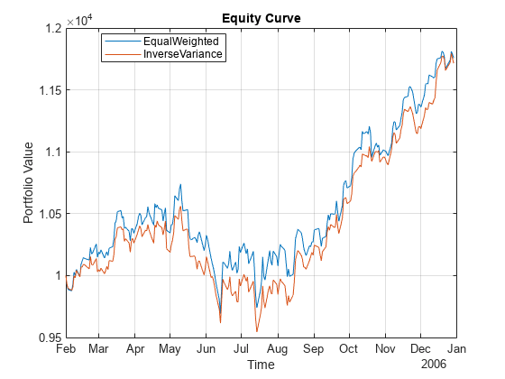
Generate Equity Curve
Use equityCurve to plot the equity curve for the equal weighted and inverse variance strategies.
equityCurve(backtester)
Rebalance Functions
This section contains the implementation of the strategy rebalance functions. For more information on creating strategies and writing rebalance functions, see backtestStrategy.
function new_weights = equalWeightFcn(current_weights, pricesTT) %#ok<INUSL>
% Equal weighted portfolio allocation

nAssets = size(pricesTT, 2);
new_weights = ones(1,nAssets);
new_weights = new_weights / sum(new_weights);

end
function new_weights = inverseVarianceFcn(current_weights, pricesTT) %#ok<INUSL>
% Inverse-variance portfolio allocation

assetReturns = tick2ret(pricesTT);
assetCov = cov(assetReturns{:,:});
new_weights = 1 ./ diag(assetCov);
new_weights = new_weights / sum(new_weights);

end
Input Arguments
Output Arguments
Version History
Introduced in R2020b
See Also
backtestStrategy | backtestEngine | runBacktest | equityCurve