simByTransition
Simulate Bates sample paths with transition
density
Description
[
simulates Paths,Times] = simByTransition(MDL,NPeriods)NTrials of Bates bivariate models driven by two
Brownian motion sources of risk and one compound Poisson process representing the
arrivals of important events over NPeriods consecutive
observation periods. simByTransition approximates continuous-time
stochastic processes by the transition density.
[
specifies options using one or more name-value pair arguments in addition to the
input arguments in the previous syntax.Paths,Times] = simByTransition(___,Name,Value)
You can perform quasi-Monte Carlo simulations using the name-value arguments for
MonteCarloMethod, QuasiSequence, and
BrownianMotionMethod. For more information, see Quasi-Monte Carlo Simulation.
Examples
Simulate Bates sample paths with transition density.
Define the parameters for the bates object.
AssetPrice = 80;
Return = 0.03;
JumpMean = 0.02;
JumpVol = 0.08;
JumpFreq = 0.1;
V0 = 0.04;
Level = 0.05;
Speed = 1.0;
Volatility = 0.2;
Rho = -0.7;
StartState = [AssetPrice;V0];
Correlation = [1 Rho;Rho 1];
Create a bates object.
batesObj = bates(Return, Speed, Level, Volatility,...
                JumpFreq, JumpMean, JumpVol,'startstate',StartState,...
                'correlation',Correlation)
batesObj =
   Class BATES: Bates Bivariate Stochastic Volatility
   --------------------------------------------------
     Dimensions: State = 2, Brownian = 2
   --------------------------------------------------
      StartTime: 0
     StartState: 2x1 double array
    Correlation: 2x2 double array
          Drift: drift rate function F(t,X(t))
      Diffusion: diffusion rate function G(t,X(t))
     Simulation: simulation method/function simByEuler
         Return: 0.03
          Speed: 1
          Level: 0.05
     Volatility: 0.2
       JumpFreq: 0.1
       JumpMean: 0.02
        JumpVol: 0.08
Define the simulation parameters.
nPeriods = 5;   % Simulate sample paths over the next five years
Paths = simByTransition(batesObj,nPeriods);
Paths
Paths = 6×2
80.0000 0.0400
99.5724 0.0201
124.2066 0.0176
56.5051 0.1806
80.4545 0.1732
94.7887 0.1169
This example shows how to use simByTransition with a Bates model to perform a quasi-Monte Carlo simulation. Quasi-Monte Carlo simulation is a Monte Carlo simulation that uses quasi-random sequences instead pseudo random numbers.
Define the parameters for the bates object.
AssetPrice = 80;
Return = 0.03;
JumpMean = 0.02;
JumpVol = 0.08;
JumpFreq = 0.1;
V0 = 0.04;
Level = 0.05;
Speed = 1.0;
Volatility = 0.2;
Rho = -0.7;
StartState = [AssetPrice;V0];
Correlation = [1 Rho;Rho 1];
Create a bates object.
Bates = bates(Return, Speed, Level, Volatility,...
                JumpFreq, JumpMean, JumpVol,'startstate',StartState,...
                'correlation',Correlation)
Bates =
   Class BATES: Bates Bivariate Stochastic Volatility
   --------------------------------------------------
     Dimensions: State = 2, Brownian = 2
   --------------------------------------------------
      StartTime: 0
     StartState: 2x1 double array
    Correlation: 2x2 double array
          Drift: drift rate function F(t,X(t))
      Diffusion: diffusion rate function G(t,X(t))
     Simulation: simulation method/function simByEuler
         Return: 0.03
          Speed: 1
          Level: 0.05
     Volatility: 0.2
       JumpFreq: 0.1
       JumpMean: 0.02
        JumpVol: 0.08
Perform a quasi-Monte Carlo simulation by using simByTransition with the optional name-value argument for 'MonteCarloMethod', 'QuasiSequence', and 'BrownianMotionMethod'.
[paths,time] = simByTransition(Bates,10,'ntrials',4096,'MonteCarloMethod','quasi','QuasiSequence','sobol','BrownianMotionMethod','brownian-bridge');
Input Arguments
Stochastic differential equation model, specified as a
bates object. For more information on creating a
bates object, see bates.
Data Types: object
Number of simulation periods, specified as a positive scalar integer. The
value of NPeriods determines the number of rows of the
simulated output series.
Data Types: double
Name-Value Arguments
Specify optional pairs of arguments as
Name1=Value1,...,NameN=ValueN, where Name is
the argument name and Value is the corresponding value.
Name-value arguments must appear after other arguments, but the order of the
pairs does not matter.
Before R2021a, use commas to separate each name and value, and enclose
Name in quotes.
Example: [Paths,Times] =
simByTransition(Bates,NPeriods,'DeltaTime',dt)
Simulated trials (sample paths) of NPeriods
observations each, specified as the comma-separated pair consisting of
'NTrials' and a positive scalar integer.
Data Types: double
Positive time increments between observations, specified as the
comma-separated pair consisting of 'DeltaTime' and a
scalar or NPeriods-by-1 column
vector.
DeltaTime represents the familiar
dt found in stochastic differential equations,
and determines the times at which the simulated paths of the output
state variables are reported.
Data Types: double
Number of intermediate time steps within each time increment
dt (defined as DeltaTime),
specified as the comma-separated pair consisting of
'NSteps' and a positive scalar integer.
The simByTransition function partitions each time
increment dt into NSteps
subintervals of length dt/NSteps,
and refines the simulation by evaluating the simulated state vector at
NSteps − 1 intermediate points. Although
simByTransition does not report the output state
vector at these intermediate points, the refinement improves accuracy by
enabling the simulation to more closely approximate the underlying
continuous-time process.
Data Types: double
Flag for storage and return method that indicates how the output array
Paths is stored and returned, specified as the
comma-separated pair consisting of 'StorePaths' and a
scalar logical flag with a value of True or
False.
If
StorePathsisTrue(the default value) or is unspecified, thensimByTransitionreturnsPathsas a three-dimensional time series array.If
StorePathsisFalse(logical0), thensimByTransitionreturns thePathsoutput array as an empty matrix.
Data Types: logical
Monte Carlo method to simulate stochastic processes, specified as the
comma-separated pair consisting of 'MonteCarloMethod'
and a string or character vector with one of the following values:
"standard"— Monte Carlo using pseudo random numbers"quasi"— Quasi-Monte Carlo using low-discrepancy sequences"randomized-quasi"— Randomized quasi-Monte Carlo
Data Types: string | char
Low discrepancy sequence to drive the stochastic processes, specified
as the comma-separated pair consisting of
'QuasiSequence' and a string or character vector
with the following value:
"sobol"— Quasi-random low-discrepancy sequences that use a base of two to form successively finer uniform partitions of the unit interval and then reorder the coordinates in each dimension
Note
If MonteCarloMethod option is not specified
or specified as"standard",
QuasiSequence is ignored.
Data Types: string | char
Brownian motion construction method, specified as the comma-separated
pair consisting of 'BrownianMotionMethod' and a
string or character vector with one of the following values:
"standard"— The Brownian motion path is found by taking the cumulative sum of the Gaussian variates."brownian-bridge"— The last step of the Brownian motion path is calculated first, followed by any order between steps until all steps have been determined."principal-components"— The Brownian motion path is calculated by minimizing the approximation error.
The starting point for a Monte Carlo simulation is the construction of a Brownian motion sample path (or Wiener path). Such paths are built from a set of independent Gaussian variates, using either standard discretization, Brownian-bridge construction, or principal components construction.
Both standard discretization and Brownian-bridge construction share
the same variance and, therefore, the same resulting convergence when
used with the MonteCarloMethod using pseudo random
numbers. However, the performance differs between the two when the
MonteCarloMethod option
"quasi" is introduced, with faster convergence
for the "brownian-bridge" construction option and the
fastest convergence for the "principal-components"
construction option.
Data Types: string | char
Sequence of end-of-period processes or state vector adjustments,
specified as the comma-separated pair consisting of
'Processes' and a function or cell array of
functions of the form
simByTransition applies processing functions at the
end of each observation period. The processing functions accept the
current observation time t and the current state
vector Xt,
and return a state vector that might adjust the input state.
If you specify more than one processing function,
simByTransition invokes the functions in the
order in which they appear in the cell array.
Data Types: cell | function
Output Arguments
Simulated paths of correlated state variables, returned as an
(NPeriods +
1)-by-NVars-by-NTrials
three-dimensional time series array.
For a given trial, each row of Paths is the transpose
of the state vector
Xt at time
t. When the input flag
StorePaths = False,
simByTransition returns Paths as
an empty matrix.
Observation times associated with the simulated paths, returned as an
(NPeriods + 1)-by-1 column vector.
Each element of Times is associated with the
corresponding row of Paths.
More About
There are inheritance relationships among the SDE classes.
The following figure illustrates the inheritance relationships.
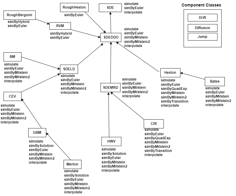
For more information, see SDE Class Hierarchy.
Transition density describes the probability distribution of a state variable transitioning from one state to another over a given time interval.
The CIR SDE has no solution such that r(t) = f(r(0),⋯).
In other words, the equation is not explicitly solvable. However, the transition density for the process is known.
The exact simulation for the distribution of r(t_1 ),⋯,r(t_n) is that of the process at times t_1,⋯,t_n for the same value of r(0). The transition density for this process is known and is expressed as
Bates models are bivariate composite models.
Each Bates model consists of two coupled univariate models:
A geometric Brownian motion (
gbm) model with a stochastic volatility function and jumps.This model usually corresponds to a price process whose volatility (variance rate) is governed by the second univariate model.
A Cox-Ingersoll-Ross (
cir) square root diffusion model.This model describes the evolution of the variance rate of the coupled Bates price process.
References
[1] Glasserman, Paul Monte Carlo Methods in Financial Engineering, New York: Springer-Verlag, 2004.
[2] Van Haastrecht, Alexander, and Antoon Pelsser. "Efficient, Almost Exact Simulation of the Heston Stochastic Volatility Model." International Journal of Theoretical and Applied Finance, Vol. 13, No. 01 (2010): 1–43.
Version History
Introduced in R2020bPerform Brownian bridge and principal components construction using the name-value
argument BrownianMotionMethod.
Perform Quasi-Monte Carlo simulation using the name-value arguments
MonteCarloMethod and
QuasiSequence.
MATLAB Command
You clicked a link that corresponds to this MATLAB command:
Run the command by entering it in the MATLAB Command Window. Web browsers do not support MATLAB commands.
选择网站
选择网站以获取翻译的可用内容,以及查看当地活动和优惠。根据您的位置,我们建议您选择:。
您也可以从以下列表中选择网站:
如何获得最佳网站性能
选择中国网站(中文或英文)以获得最佳网站性能。其他 MathWorks 国家/地区网站并未针对您所在位置的访问进行优化。
美洲
- América Latina (Español)
- Canada (English)
- United States (English)
欧洲
- Belgium (English)
- Denmark (English)
- Deutschland (Deutsch)
- España (Español)
- Finland (English)
- France (Français)
- Ireland (English)
- Italia (Italiano)
- Luxembourg (English)
- Netherlands (English)
- Norway (English)
- Österreich (Deutsch)
- Portugal (English)
- Sweden (English)
- Switzerland
- United Kingdom (English)