Forecasting Corporate Default Rates

This example shows how to build a forecasting model for corporate default rates.

Risk parameters are dynamic in nature, and understanding how these parameters change in time is a fundamental task for risk management.

In the first part of this example, we work with historical credit migrations data to construct some time series of interest, and to visualize default rates dynamics. In the second part of this example, we use some of the series constructed in the first part, and some additional data, to fit a forecasting model for corporate default rates, and to show some backtesting and stress testing concepts. A linear regression model for corporate default rates is presented, but the tools and concepts described can be used with other forecasting methodologies. The appendix at the end references the handling of models for full transition matrices.

People interested in forecasting, backtesting, and stress testing can go directly to the second part of this example. The first part of this example is more relevant for people who work with credit migration data.

Part I: Working with Credit Migrations Data

We work with historical transition probabilities for corporate issuers (variable TransMat). This is yearly data for the period 1981-2005, from [10]. The data includes, for each year, the number of issuers per rating at the beginning of the year (variable nIssuers), and the number of new issuers per rating per year (variable nNewIssuers). There is also a corporate profits forecast, from [9], and a corporate spread, from [4] (variables CPF and SPR). A variable indicating recession years (Recession), consistent with recession dates from [7], is used mainly for visualizations.

Example_LoadData

Getting Default Rates for Different Ratings Categories

We start by performing some aggregations to get corporate default rates for Investment Grade (IG) and Speculative Grade (SG) issuers, and the overall corporate default rate.

Aggregation and segmentation are relative terms. IG is an aggregate with respect to credit ratings, but a segment from the perspective of the overall corporate portfolio. Other segments are of interest in practice, for example, economic sectors, industries, or geographic regions. The data we use, however, is aggregated by credit ratings, so further segmentation is not possible. Nonetheless, the tools and workflow discussed here can be useful to work with other segment-specific models.

Use functionality in Financial Toolbox™, specifically, the functions transprobgrouptotals and transprobbytotals, to perform the aggregation. These functions take as inputs structures with credit migration information in a particular format. We set up the inputs here and visualize them below to understand their information and format.

% Pre-allocate the struct array
totalsByRtg(nYears,1) = struct('totalsVec',[],'totalsMat',[],...
   'algorithm','cohort');
for t = 1:nYears
   % Number of issuers per rating at the beginning of the year
   totalsByRtg(t).totalsVec = nIssuers(t,:);
   % Number of transitions between ratings during the year
   totalsByRtg(t).totalsMat = round(diag(nIssuers(t,:))*...
      (0.01*TransMat(:,:,t)));
   % Algorithm
   totalsByRtg(t).algorithm = 'cohort';
end

It is useful to see both the original data and the data stored in these totals structures side to side. The original data contains number of issuers and transition probabilities for each year. For example, for 2005:

fprintf('\nTransition matrix for 2005:\n\n')

Transition matrix for 2005:

Example_DisplayTransitions(squeeze(TransMat(:,:,end)),nIssuers(end,:),...
   {'AAA','AA','A','BBB','BB','B','CCC'},...
   {'AAA','AA','A','BBB','BB','B','CCC','D','NR'})

         Init    AAA     AA      A    BBB     BB      B    CCC      D     NR 
   AAA     98  88.78   9.18   1.02      0      0      0      0      0   1.02 
    AA    407      0  90.66   4.91   0.49      0      0      0      0   3.93 
     A   1224   0.08   1.63  88.89   4.41      0      0      0      0   4.98 
   BBB   1535      0    0.2   5.93  84.04   3.06   0.46      0   0.07   6.25 
    BB   1015      0      0      0   5.71  76.75    6.9    0.2    0.2  10.25 
     B   1010      0      0    0.1   0.59   8.51  70.59   3.76   1.58  14.85 
   CCC    126      0      0      0   0.79   0.79   25.4  46.83   8.73  17.46

The totals structure stores the total number of issuers per rating at the beginning of the year in the totalsVec field, and the total number of migrations between ratings (instead of transition probabilities) in the totalsMat field. Here is the information for 2005:

fprintf('\nTransition counts (totals struct) for 2005:\n\n')

Transition counts (totals struct) for 2005:

Example_DisplayTransitions(totalsByRtg(end).totalsMat,...
   totalsByRtg(end).totalsVec,...
   {'AAA','AA','A','BBB','BB','B','CCC'},...
   {'AAA','AA','A','BBB','BB','B','CCC','D','NR'})

         Init    AAA     AA      A    BBB     BB      B    CCC      D     NR 
   AAA     98     87      9      1      0      0      0      0      0      1 
    AA    407      0    369     20      2      0      0      0      0     16 
     A   1224      1     20   1088     54      0      0      0      0     61 
   BBB   1535      0      3     91   1290     47      7      0      1     96 
    BB   1015      0      0      0     58    779     70      2      2    104 
     B   1010      0      0      1      6     86    713     38     16    150 
   CCC    126      0      0      0      1      1     32     59     11     22

The third field in the totals structure, algorithm, indicates that we are working with the cohort method (duration is also supported, although the information in totalsVec and totalsMat would be different). These structures are obtained as optional outputs from transprob, but this example shows how you can define these structures directly.

Use transprobgrouptotals to group the ratings 'AAA' to 'BBB' (ratings 1 to 4) into the IG category and ratings 'BB' to 'CCC' (ratings 5 to 7) into the SG category. The edges argument tells the function which ratings are to be grouped together (1 to 4, and 5 to 7). We also group all non-default ratings into one category. These are preliminary steps to get the IG, SG, and overall default rates for each year.

edgesIGSG = [4 7];
totalsIGSG = transprobgrouptotals(totalsByRtg,edgesIGSG);
edgesAll = 7; % could also use edgesAll = 2 with totalsIGSG
totalsAll = transprobgrouptotals(totalsByRtg,edgesAll);

Here are the 2005 totals grouped at IG/SG level, and the corresponding transition matrix, recovered using transprobbytotals.

fprintf('\nTransition counts for 2005 at IG/SG level:\n\n')

Transition counts for 2005 at IG/SG level:

Example_DisplayTransitions(totalsIGSG(end).totalsMat,...
   totalsIGSG(end).totalsVec,...
   {'IG','SG'},...
   {'IG','SG','D','NR'})

         Init     IG     SG      D     NR 
    IG   3264   3035     54      1    174 
    SG   2151     66   1780     29    276

fprintf('\nTransition matrix for 2005 at IG/SG level:\n\n')

Transition matrix for 2005 at IG/SG level:

Example_DisplayTransitions(transprobbytotals(totalsIGSG(end)),[],...
   {'IG','SG'},...
   {'IG','SG','D','NR'})

           IG     SG      D     NR 
    IG  92.98   1.65   0.03   5.33 
    SG   3.07  82.75   1.35  12.83

Now get transition matrices for every year both at IG/SG and non-default/default levels and store the default rates only (we do not use the rest of the transition probabilities).

DefRateIG = zeros(nYears,1);
DefRateSG = zeros(nYears,1);
DefRate = zeros(nYears,1);
for t=1:nYears
   % Get transition matrix at IG/SG level and extract IG default rate and
   % SG default rate for year t
   tmIGSG = transprobbytotals(totalsIGSG(t));
   DefRateIG(t) = tmIGSG(1,3);
   DefRateSG(t) = tmIGSG(2,3);
   % Get transition matrix at most aggregate level and extract overall
   % corporate default rate for year t
   tmAll = transprobbytotals(totalsAll(t));
   DefRate(t) = tmAll(1,2);
end

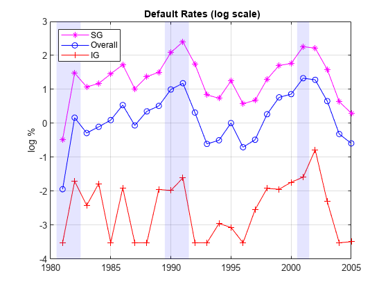
Here is a visualization of the dynamics of IG, SG, and overall corporate default rates together. To emphasize their patterns, rather than their magnitudes, a log scale is used. The shaded bands indicate recession years. The patterns of SG and IG are slightly different. For example, the IG rate is higher in 1994 than in 1995, but the opposite is true for SG. More noticeably, the IG default rate peaked after the 2001 recession, in 2002, whereas the peak for SG is in 2001. This suggests that models for the dynamics of the IG and SG default rates could have important differences, a common situation when working with different segments. The overall corporate default rate is by construction a combination of the other two, and its pattern is closer to SG, most likely due to the relative magnitude of SG versus IG.

minIG = min(DefRateIG(DefRateIG~=0));
figure
plot(Years,log(DefRateSG),'m-*')
hold on
plot(Years,log(DefRate),'b-o')
plot(Years,log(max(DefRateIG,minIG-0.001)),'r-+')
Example_RecessionBands
hold off
grid on
title('{\bf Default Rates (log scale)}')
ylabel('log %')
legend({'SG','Overall','IG'},'location','NW')

Figure contains an axes object. The axes object with title blank Default blank Rates blank (log blank scale), ylabel log % contains 8 objects of type line, patch. These objects represent SG, Overall, IG.

Getting Default Rates for Different Time Periods

The default rates obtained are examples of point-in-time (PIT) rates, only the most recent information is used to estimate them. On the other extreme, we can use all the migrations observed in the 25 years spanned by the dataset to estimate long-term, or through-the-cycle (TTC) default rates. Other rates of interest are the average default rates over recession or expansion years.

All of these are easy to estimate with the data we have and the same tools. For example, to estimate the average transition probabilities over recession years, pass to transprobbytotals the totals structures corresponding to the recession years only. We use logical indexing below, taking advantage of the Recession variable. transprobbytotals aggregates the information over time and returns the corresponding transition matrix.

tmAllRec = transprobbytotals(totalsAll(Recession));
DefRateRec = tmAllRec(1,2);

tmAllExp = transprobbytotals(totalsAll(~Recession));
DefRateExp = tmAllExp(1,2);

tmAllTTC = transprobbytotals(totalsAll);
DefRateTTC = tmAllTTC(1,2);

The following figure shows the estimated PIT rates, TTC rates, and recession and expansion rates.

DefRateTwoValues = DefRateExp*ones(nYears,1);
DefRateTwoValues(Recession) = DefRateRec;

figure
plot(Years,DefRate,'bo:','LineWidth',1.2)
hold on
stairs(Years-0.5,DefRateTwoValues,'m-','LineWidth',1.5)
plot(Years,DefRateTTC*ones(nYears,1),'r-.','LineWidth',1.5)
Example_RecessionBands
hold off
grid on
title('{\bf Default Rate}')
ylabel('%')
legend({'Point-in-time (PIT)','Recession/Expansion Avg',...
   'Through-the-cycle (TTC)'},'location','NW')

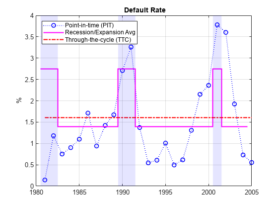
Figure contains an axes object. The axes object with title blank Default blank Rate, ylabel % contains 8 objects of type line, stair, patch. These objects represent Point-in-time (PIT), Recession/Expansion Avg, Through-the-cycle (TTC).

Some analyses (see, for example, [11]) use simulations where the default rate is conditional on the general state of the economy, for example, recession v. expansion. The recession and expansion estimates obtained can be useful in such a framework. These are all historical averages, however, and may not work well if used as predictions for the actual default rates expected on any particular year. In the second part of this example, we revisit the use of these types of historical averages as forecasting tools in a backtesting exercise.

Building Predictors Using Credit Ratings Data

Using the credit data, you can build new time series of interest. We start with an age proxy that is used as predictor in the forecasting model in the second part of this example.

Age is known to be an important factor in predicting default rates; see, for example, [1] and [5]. Age here means the number of years since a bond was issued. By extension, the age of a portfolio is the average age of its bonds. Certain patterns have been observed historically. Many low-quality borrowers default just a few years after issuing a bond. When troubled companies issue bonds, the amount borrowed helps them make payments for a year or two. Beyond that point, their only source of money is their cash flows, and if they are insufficient, default occurs.

We cannot calculate the exact age of the portfolio, because there is no information at issuer level in the dataset. We follow [6], however, and use the number of new issuers in year t-3 divided by the total number of issuers at the end of year t as an age proxy. Because of the lag, the age proxy starts in 1984. For the numerator, we have explicit information on the number of new issuers. For the denominator, the number of issuers at the end of a year equals the number of issuers at the beginning of next year. This is known for all years but the last one, which is set to the total transitions into a non-default rating plus the number of new issuers on that year.

% Total number of issuers at the end of the year
nEOY = zeros(nYears,1);
% nIssuers is number of issuers per ratings at the beginning of the year
% nEOY ( 1981 ) = sum nIssuers ( 1982 ), etc until 2004
nEOY(1:end-1) = sum(nIssuers(2:end,:),2);
% nEOY ( 2005 ) = issuers in non-default state at end of 2005 plus
% new issuers in 2005
nEOY(end) = totalsAll(end).totalsMat(1,1) + sum(nNewIssuers(end,:));
% Age proxy
AGE = 100*[nan(3,1); sum(nNewIssuers(1:end-3,:),2)./nEOY(4:end)];

Examples of other time series of interest are the proportion of SG issuers at the end of each year, or an age proxy for SG.

% nSGEOY: Number of SG issuers at the end of the year
% nSGEOY is similar to nEOY, but for SG only, from 5 ('BB') to 7 ('CCC')
indSG = 5:7;
nSGEOY = zeros(nYears,1);
nSGEOY(1:end-1) = sum(nIssuers(2:end,indSG),2);
nSGEOY(end) = sum(totalsIGSG(end).totalsMat(:,2)) +...
   sum(nNewIssuers(end,indSG));
% Proportion of SG issuers
SG = 100*nSGEOY./nEOY;
% SG age proxy: new SG issuers in t-3 / total issuers at the end of year t
AGESG = 100*[nan(3,1); sum(nNewIssuers(1:end-3,indSG),2)./nEOY(4:end)];

Part II: A Forecasting Model for Default Rates

We work with the following linear regression model for corporate default rates

$D e f R a t e = β_{0} + β_{a g e} A G E + β_{c p f} C P F + β_{s p r} S P R$

where

AGE: Age proxy defined above
CPF: Corporate profits forecast
SPR: Corporate spread over treasuries

This is the same model as in [6], except the model in [6] is for IG only.

As previously discussed, age is known to be an important factor regarding default rates. The corporate profits provide information on the economic environment. The corporate spread is a proxy for credit quality. Age, environment, and quality are three dimensions frequently found in credit analysis models.

inSample = 4:nYears-1;
T = length(inSample);
varNames = {'AGE','CPF','SPR'};
X = [AGE CPF SPR];
X = X(inSample,:);
y = DefRate(inSample+1); % DefaultRate, year t+1
stats = regstats(y,X);

fprintf('\nConst   AGE   CPF   SPR   adjR^2\n')

Const   AGE   CPF   SPR   adjR^2

fprintf('%1.2f  %1.2f %1.2f  %1.2f   %1.4f\n',...
   [stats.beta;stats.adjrsquare])

-1.19  0.15 -0.10  0.71   0.7424

The coefficients have the expected sign: default rates tend to increase with a higher proportion of 3-year issuers, decrease with good corporate profits, and increase when the corporate yields are higher. The adjusted R square shows a good fit.

The in-sample fit, or how close the model predictions are from the sample points used to fit the model, is shown in the following figure.

bHat = stats.beta;
yHat = [ones(T,1),X]*bHat;

figure
plot(Years(inSample+1),DefRate(inSample+1),'ko','LineWidth',1.5,...
   'MarkerSize',10,'MarkerFaceColor','g')
hold on
plot(Years(inSample+1),yHat,'b-s','LineWidth',1.2,'MarkerSize',10)
hold off
grid on
legend({'Actual','Model'},'location','NW')
title('{\bf Corporate Default Rate Models: In-Sample Fit}')
xlabel('Year')
ylabel('Percent')

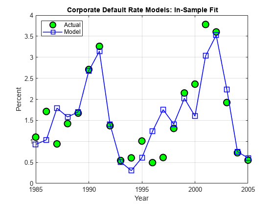
Figure contains an axes object. The axes object with title blank Corporate blank Default blank Rate blank Models: blank In-Sample blank Fit, xlabel Year, ylabel Percent contains 2 objects of type line. One or more of the lines displays its values using only markers These objects represent Actual, Model.

It can be shown that there is no strong statistical evidence to conclude that the linear regression assumptions are violated. It is apparent that default rates are not normally distributed. The model, however, does not make that assumption. The only normality assumption in the model is that, given the predictors values, the error between the predicted and the observed default rates is normally distributed. By looking at the in-sample fit, this does not seem unreasonable. The magnitude of the errors certainly seems independent of whether the default rates are high or low. Year 2001 has a high default rate and a high error, but years 1991 or 2002 also have high rates and yet very small errors. Likewise, low default rate years like 1996 and 1997 show considerable errors, but years 2004 or 2005 have similarly low rates and tiny errors.

A thorough statistical analysis of the model is out of scope here, but there are several detailed examples in Statistics and Machine Learning Toolbox™ and Econometrics Toolbox™.

Backtesting

To evaluate how this model performs out-of-sample, we set up a backtesting exercise. Starting at the end of 1995, we fit the linear regression model with the information available up to that date, and compare the model prediction to the actual default rate observed the following year. We repeat the same for all subsequent years until the end of the sample.

For backtesting, relative performance of a model, when compared to alternatives, is easier to assess than the performance of a model in isolation. Here we include two alternatives to determine next year's default rate, both likely candidates in practice. One is the TTC default rate, estimated with data from the beginning of the sample to the current year, a very stable default rate estimate. The other is the PIT rate, estimated using data from the most recent year only, much more sensitive to recent events.

XBT = [AGE,CPF,SPR];
yBT = DefRate;

iYear0 = find(Years==1984); % index of first year in sample, 1984
T = find(Years==1995); % ind "current" year, start at 1995, updated in loop
YearsBT = 1996:2005; % years predicted in BT exercise
iYearsBT = find(Years==1996):find(Years==2005); % corresponding indices
nYearsBT = length(YearsBT); % number of years in BT exercise

MethodTags = {'Model','PIT','TTC'};
nMethods = length(MethodTags);
PredDefRate = zeros(nYearsBT,nMethods);
ErrorBT = zeros(nYearsBT,nMethods);

alpha = 0.05;
PredDefLoBnd = zeros(nYearsBT,1);
PredDefUpBnd = zeros(nYearsBT,1);

for k=1:nYearsBT
   % In sample years for predictors, from 1984 to "last" year (T-1)
   inSampleBT = iYear0:T-1;
   
   % Method 1: Linear regression model
   %   Fit regression model with data up to "current" year (T)
   s = regstats(yBT(inSampleBT+1),XBT(inSampleBT,:));
   %   Predict default rate for "next" year (T+1)
   PredDefRate(k,1) = [1 XBT(T,:)]*s.beta;
   %   Compute prediction intervals
   tCrit = tinv(1-alpha/2,s.tstat.dfe);
   PredStd = sqrt([1 XBT(T,:)]*s.covb*[1 XBT(T,:)]'+s.mse);
   PredDefLoBnd(k) = max(0,PredDefRate(k,1) - tCrit*PredStd);
   PredDefUpBnd(k) = PredDefRate(k,1) + tCrit*PredStd;

   % Method 2: Point-in-time (PIT) default rate
   PredDefRate(k,2) = DefRate(T);

   % Method 3: Through-the-cycle (TTC) default rate
   tmAll = transprobbytotals(totalsAll(iYear0:T));
   PredDefRate(k,3) = tmAll(1,2);

   % Update error
   ErrorBT(k,:) = PredDefRate(k,:) - DefRate(T+1);
   
   % Move to next year
   T = T + 1;
end

Here are the predictions of the three alternative approaches, compared to the actual default rates observed. Unsurprisingly, TTC shows a very poor predictive power. However, it is not obvious whether PIT or the linear regression model makes better predictions in this 10-year time span.

Example_BacktestPlot(YearsBT,DefRate(iYearsBT),PredDefRate,'Year','%',...
   '{\bf Default Rate Estimation Methods: Backtesting}',...
   ['Actual' MethodTags],'NW')

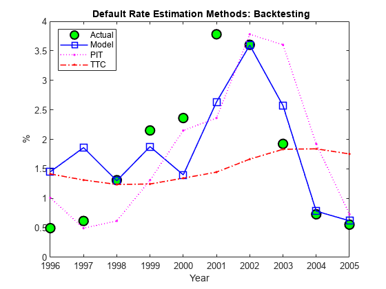
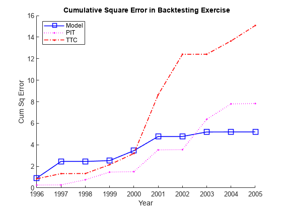
Figure contains an axes object. The axes object with title blank Default blank Rate blank Estimation blank Methods: blank Backtesting, xlabel Year, ylabel % contains 4 objects of type line. One or more of the lines displays its values using only markers These objects represent Actual, Model, PIT, TTC.

The following plot keeps track of cumulative square error, a measure often used for comparisons in backtesting exercises. This confirms TTC as a poor alternative. PIT shows lower cumulative error than the linear regression model in the late nineties, but after the 2001 recession the situation is reversed. Cumulative square error, however, is not an intuitive measure, it is hard to get a sense of what the difference between these alternatives means in practical terms.

CumSqError = cumsum(ErrorBT.^2);
Example_BacktestPlot(YearsBT,[],CumSqError,'Year','Cum Sq Error',...
   '{\bf Cumulative Square Error in Backtesting Exercise}',...
   MethodTags,'NW')

Figure contains an axes object. The axes object with title blank Cumulative blank Square blank Error blank in blank Backtesting blank Exercise, xlabel Year, ylabel Cum Sq Error contains 3 objects of type line. These objects represent Model, PIT, TTC.

It makes sense to translate the prediction errors into a monetary measure. Here we measure the impact of the prediction error on a simplified framework for generating loss reserves in an institution.

We assume a homogeneous portfolio, where all credits have the same probability of default, the same loss given default (LGD), and the same exposure at default (EAD). Both LGD and EAD are assumed to be known. For simplicity, we keep these values constant for the 10 years of the exercise. We set LGD at 45%, and EAD per bond at 100 million. The portfolio is assumed to have a thousand bonds, so the total value of the portfolio, the total EAD, is 100 billion.

The predicted default rate for year t, determined at the end of year t-1, is used to calculate the expected loss for year t

$E L_{t} = E A D_{t} \times L G D_{t} \times P r e d i c t e d D e f a u l t R a t e_{t}$

This is the amount added to the loss reserves at the start of year t. At the end of the year, the actual losses are known

$A L_{t} = E A D_{t} \times L G D_{t} \times O b s e r v e d D e f a u l t R a t e_{t}$

We assume that unused loss reserves remain in the reserves fund. The starting balance in reserves at the beginning of the exercise is set to zero. If the actual losses surpass the expected loss, unused reserves accumulated over the years are used first, and only if these run out, capital is used to cover a shortfall. All this translates into the following formula

$R e s e r v e s_{t} = R e s e r v e s_{t - 1} + (E L_{t} - A L_{t})$

or equivalently

$R e s e r v e s_{t} = \sum_{s = 1}^{t} (E L_{t} - A L_{t})$

The following figure shows the loss reserves balance for each of the three alternatives in the backtesting exercise.

EAD = 100*ones(nYearsBT,1); % in billions
LGD = 0.45*ones(nYearsBT,1); % Loss given default, 45%
% Reserves excess or shortfall for each year, in billions
ReservesExcessShortfall = bsxfun(@times,EAD.*LGD,ErrorBT/100);
% Cumulative reserve balance for each year, in billions
ReservesBalanceEOY = cumsum(ReservesExcessShortfall);

Example_BacktestPlot(YearsBT,[],ReservesBalanceEOY,'Year',...
   'Billions of Dollars',...
   '{\bf Reserves Balance (EOY): Backtesting}',...
   MethodTags,'SW')
grid on

Figure contains an axes object. The axes object with title blank Reserves blank Balance blank (EOY): blank Backtesting, xlabel Year, ylabel Billions of Dollars contains 3 objects of type line. These objects represent Model, PIT, TTC.

Using the linear regression model we only observe a deficit in reserves in two out of ten years, and the maximum deficit, in 2001, is 0.09 billion, only nine basis points of the portfolio value.

In contrast, both TTC and PIT reach a deficit of 1.2 billion by 2001. Things get worse for TTC in the next two years, reaching a deficit of 2.1 billion by 2003. PIT does make a correction quickly after 2001, and by 2004 the reserves have a surplus. Yet, both TTC and PIT lead to more deficit years than surplus years in this exercise.

The linear regression model shows more of a counter-cyclical effect than the alternatives in this exercise. The money set aside using the linear regression model reaches close to a billion in 1997 and 1998. High levels of unused reserves translate into a slower pace of lending (not reflected in the exercise, because we exogenously impose the portfolio value). Moreover, capital is only slightly impacted during the 2001 recession thanks to the reserves accumulated over the previous expansion. This translates into more capital available to back up further lending, if desired, during the economic recovery.

The last backtesting tool we discuss is the use of prediction intervals. Linear regression models provide standard formulas to compute confidence intervals for the values of new observations. These intervals are shown in the next figure for the 10 years spanned in the backtesting exercise.

figure
plot(YearsBT,DefRate(iYearsBT),'ko','LineWidth',1.5,'MarkerSize',10,...
   'MarkerFaceColor','g')
hold on
plot(YearsBT,PredDefRate(:,1),'b-s','LineWidth',1.2,'MarkerSize',10)
plot(YearsBT,[PredDefLoBnd PredDefUpBnd],'b:','LineWidth',1.2)
hold off
strConf = num2str((1-alpha)*100);
title(['{\bf Backtesting Results with ' strConf '% Prediction Intervals}'])
xlabel('Year');
ylabel('%');
legend({'Actual','Predicted','Conf Bounds'},'location','NW');

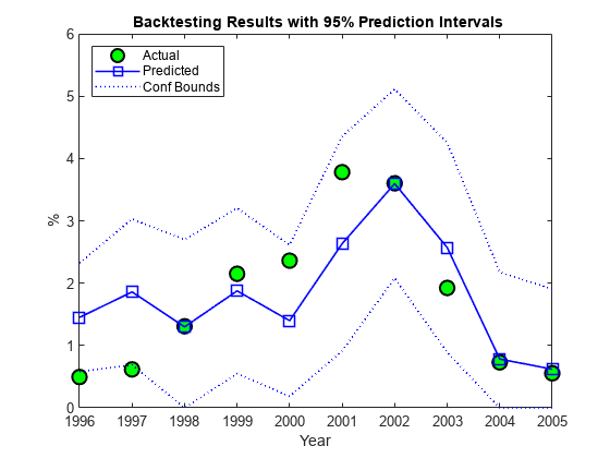
Figure contains an axes object. The axes object with title blank Backtesting blank Results blank with blank 95 % blank Prediction blank Intervals, xlabel Year, ylabel % contains 4 objects of type line. One or more of the lines displays its values using only markers These objects represent Actual, Predicted, Conf Bounds.

The observed default rates fall outside the prediction intervals for two years, 1996 and 1997, where very low default rates are observed. For a 95% confidence level, two out of 10 seems high. Yet, the observed values in these cases fall barely outside the prediction interval, which is a positive sign for the model. It is also positive that the prediction intervals contain the observed values around the 2001 recession.

Stress Testing

Stress testing is a broad area that reaches far beyond computational tools; see, for example, [3]. We show some tools that can be incorporated into a comprehensive stress testing framework. We build on the linear regression model presented above, but the concepts and tools are compatible with other forecasting methodologies.

The first tool is the use of prediction intervals to define a worst-case scenario forecasts. This is to account for uncertainty in the model only, not in the value of the predictors.

We take a baseline scenario of predictors, in our case, the latest known values of our age proxy AGE, corporate profits forecast, CPF, and corporate spread, SPR. We then use the linear regression model to compute a 95% confidence upper bound for the predicted default rate. The motivation for this is illustrated in the last plot of the backtesting section, where the 95% confidence upper limit acts as a conservative bound when the prediction underestimates the actual default rates.

tCrit = tinv(1-alpha/2,stats.tstat.dfe);
XLast = [AGE(end),CPF(end),SPR(end)];

yPred = [1 XLast]*stats.beta;
PredStd = sqrt([1 XLast]*stats.covb*[1 XLast]'+stats.mse);
yPredUB = yPred + tCrit*PredStd;

fprintf('\nPredicted default rate:\n');

Predicted default rate:

fprintf('     Baseline: %4.2f%%\n',yPred);

     Baseline: 1.18%

fprintf('     %g%% Upper Bound: %4.2f%%\n',(1-alpha)*100,yPredUB);

     95% Upper Bound: 2.31%

The next step is to incorporate stressed scenarios of the predictors in the analysis. CPF and SPR can change in the short term, whereas AGE cannot. This is important. The corporate profits forecast and the corporate spread are influenced by world events, including, for example, natural disasters. These predictors can significantly change overnight. On the other hand, AGE depends on managerial decisions that can alter the proportion of old and new loans in time, but these decisions take months, if not years, to reflect in the AGE time series. Scenarios for AGE are compatible with longer term analyses. Here we look at one year ahead only, and keep AGE fixed for the remainder of this section.

It is convenient to define the predicted default rate and the confidence bounds as functions of CPF and SPR to simplify the scenario analysis.

yPredFn = @(cpf,spr) [1 AGE(end) cpf spr]*stats.beta;
PredStdFn = @(cpf,spr) sqrt([1 AGE(end) cpf spr]*stats.covb*...
   [1 AGE(end) cpf spr]'+stats.mse);
yPredUBFn = @(cpf,spr) (yPredFn(cpf,spr) + tCrit*PredStdFn(cpf,spr));
yPredLBFn = @(cpf,spr) (yPredFn(cpf,spr) - tCrit*PredStdFn(cpf,spr));

Two extreme scenarios of interest can be a drop in the corporate profits forecast of 4% relative to the baseline, and an increase in the corporate spread of 100 basis points over the baseline.

Moving one predictor at a time is not unreasonable in this case, because the correlation between CPF and SPR is very low. Moderate correlation levels may require perturbing predictors together to get more reliable results. Highly correlated predictors usually do not coexist in the same model, since they offer redundant information.

fprintf('\n\n         What-if Analysis\n');

         What-if Analysis

fprintf('Scenario         LB    Pred    UB\n');

Scenario         LB    Pred    UB

cpf = CPF(end)-4;
spr = SPR(end);
yPredRange = [yPredLBFn(cpf,spr),yPredFn(cpf,spr),yPredUBFn(cpf,spr)];
fprintf('CPF drops 4%%    %4.2f%%  %4.2f%%  %4.2f%%\n',yPredRange);

CPF drops 4%    0.42%  1.57%  2.71%

cpf = CPF(end);
spr = SPR(end)+1;
yPredRange = [yPredLBFn(cpf,spr),yPredFn(cpf,spr),yPredUBFn(cpf,spr)];
fprintf('SPR rises 1%%    %4.2f%%  %4.2f%%  %4.2f%%\n',yPredRange);

SPR rises 1%    0.71%  1.88%  3.05%

cpf = CPF(end);
spr = SPR(end);
yPredRange = [yPredLBFn(cpf,spr),yPredFn(cpf,spr),yPredUBFn(cpf,spr)];
fprintf('    Baseline    %4.2f%%  %4.2f%%  %4.2f%%\n',yPredRange);

    Baseline    0.04%  1.18%  2.31%

fprintf('\nCorrelation between CPF and SPR: %4.3f\n',corr(CPF,SPR));

Correlation between CPF and SPR: 0.012

We now take a more global view of the scenario analysis. Instead of analyzing one scenario at a time, we visualize the default rate forecasts as a function of CPF and SPR. More precisely, we plot default rate contours over a whole grid of CPF and SPR values. We use the conservative 95% upper bound.

If we assumed a particular bivariate distribution for the values of CPF and SPR, we could plot the contours of their distribution in the same figure. That would give visual information on the probability of falling on each region. Lacking such a distribution, we simply add to the plot the CPF - SPR pairs observed in our sample, as a historical, empirical distribution. The last observation in the sample, the baseline scenario, is marked in red.

gridCPF = 2*min(CPF):0.1:max(CPF);
gridSPR = min(SPR):0.1:2*max(SPR);
nGridCPF = length(gridCPF);
nGridSPR = length(gridSPR);

DefRateUB = zeros(nGridCPF,nGridSPR);
for i=1:nGridCPF
   for j=1:nGridSPR
      DefRateUB(i,j) = yPredUBFn(gridCPF(i),gridSPR(j));
   end
end
Example_StressTestPlot(gridCPF,gridSPR,DefRateUB,CPF,SPR,...
   'Corporate Profits Forecast (%)','Corporate Spread (%)',...
   ['{\bf ' strConf '% UB Default Rate Regions (in %)}'])

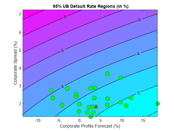
Figure contains an axes object. The axes object with title blank 95 % blank UB blank Default blank Rate blank Regions blank (in blank %), xlabel Corporate Profits Forecast (%), ylabel Corporate Spread (%) contains 3 objects of type contour, line, scatter. One or more of the lines displays its values using only markers

Very different predictor values result in similar default rate levels. For example, consider a profits forecast around 10% with a spread of 3.5%, and a profits forecast of -2.5% with a spread of 2%, they both result in a default rate slightly above 3%. Also, only one point in the available history yields a default rate higher than 4%.

Monetary terms, once again, may be more meaningful. We use the Basel II capital requirements formula (see [2]) to translate the default rates into a monetary measure. The Basel II formula is convenient because it is analytic (there is no need to simulate to estimate the capital requirements), but also because it depends only on the probabilities of default. We define the Basel II capital requirements as a function K.

% Correlation as a function of PD
w = @(pd) (1-exp(-50*pd))/(1-exp(-50)); % weight
R = @(pd) (0.12*w(pd)+0.24*(1-w(pd))); % correlation
% Vasicek formula
V = @(pd) normcdf(norminv(pd)+R(pd).*norminv(0.999)./sqrt(1-R(pd)));
% Parameter b for maturity adjustment
b = @(pd) (0.11852-0.05478*log(pd)).^2;
% Basel II capital requirement with LGD=45% and maturity M=2.5 (numerator
% in maturity adjustment term becomes 1)
K = @(pd) 0.45*(V(pd)-pd).*(1./(1-1.5*b(pd)));

Worst-case default rates for a whole grid of CPF - SPR pairs are stored in DefRateUB. By applying the function K to DefRateUB, we can visualize the capital requirements over the same grid.

CapReq = 100*K(DefRateUB/100);
Example_StressTestPlot(gridCPF,gridSPR,CapReq,CPF,SPR,...
   'Corporate Profits Forecast (%)','Corporate Spread (%)',...
   {'{\bf Capital Requirement Regions (% of value)}';...
   ['{\bf using ' strConf '% UB Default Rate}']})

Figure contains an axes object. The axes object with title blank Capital blank Requirement blank Regions blank (% blank of blank value) blank blank using blank 95 % blank UB blank Default blank Rate, xlabel Corporate Profits Forecast (%), ylabel Corporate Spread (%) contains 3 objects of type contour, line, scatter. One or more of the lines displays its values using only markers

The contour levels now indicate capital requirements as a percentage of portfolio value. The two scenarios above, profits of 10% with spread of 3.5%, and profits of -2.5% and spread of 2%, result in capital requirements near 2.75%. The worst-case point from the historical data yields a capital requirement of about 3%.

This visualization can also be used, for example, as part of a reverse stress test analysis. Critical levels of capital can be determined first, and the figure can be used to determine regions of risk factor values (in this case CPF and SPR) that lead to those critical levels.

Instead of historical observations of CPF and SPR, an empirical distribution for the risk factors can be simulated using, for example, a vector autoregressive (VAR) model from Econometrics Toolbox™. The capital requirements corresponding to each default probability level can be found by simulation if a closed form formula is not available, and the same plots can be generated. For large simulations, a distributed computing implementation using Parallel Computing Toolbox™ or MATLAB® Parallel Server™ can make the process more efficient.

Appendix: Modeling Full Transition Matrices

Transition matrices change in time, and a full description of their dynamics requires working with multi-dimensional time series. There are, however, techniques that exploit the particular structure of transition matrices to reduce the dimensionality of the problem. In [8], for example, a single parameter related to the proportion of downgrades is used, and both [6] and [8] describe a method to shift transition probabilities using a single parameter. The latter approach is shown in this appendix.

The method takes the TTC transition matrix as a baseline.

tmTTC = transprobbytotals(totalsByRtg);
Example_DisplayTransitions(tmTTC,[],...
   {'AAA','AA','A','BBB','BB','B','CCC'},...
   {'AAA','AA','A','BBB','BB','B','CCC','D','NR'})

          AAA     AA      A    BBB     BB      B    CCC      D     NR 
   AAA   88.2   7.67   0.49   0.09   0.06      0      0      0   3.49 
    AA   0.58  87.16   7.63   0.58   0.06   0.11   0.02   0.01   3.85 
     A   0.05    1.9  87.24   5.59   0.42   0.15   0.03   0.04   4.58 
   BBB   0.02   0.16   3.85  84.13   4.27   0.76   0.17   0.27   6.37 
    BB   0.03   0.04   0.25   5.26  75.74   7.36    0.9   1.12   9.29 
     B      0   0.05   0.19   0.31   5.52  72.67   4.21   5.38  11.67 
   CCC      0      0   0.28   0.41   1.24  10.92  47.06  27.02  13.06

An equivalent way to represent this matrix is by transforming it into credit quality thresholds, that is, critical values of a standard normal distribution that yield the same transition probabilities (row by row).

thresholdMat = transprobtothresholds(tmTTC);
Example_DisplayTransitions(thresholdMat,[],...
   {'AAA','AA','A','BBB','BB','B','CCC'},...
   {'AAA','AA','A','BBB','BB','B','CCC','D','NR'})

          AAA     AA      A    BBB     BB      B    CCC      D     NR 
   AAA    Inf  -1.19  -1.74   -1.8  -1.81  -1.81  -1.81  -1.81  -1.81 
    AA    Inf   2.52  -1.16  -1.68  -1.75  -1.75  -1.76  -1.77  -1.77 
     A    Inf   3.31   2.07  -1.24  -1.62  -1.66  -1.68  -1.68  -1.69 
   BBB    Inf   3.57   2.91   1.75  -1.18  -1.43  -1.49   -1.5  -1.52 
    BB    Inf   3.39   3.16   2.72   1.59  -0.89  -1.21  -1.26  -1.32 
     B    Inf    Inf   3.28   2.82   2.54   1.55   -0.8  -0.95  -1.19 
   CCC    Inf    Inf    Inf   2.77   2.46   2.07   1.13  -0.25  -1.12

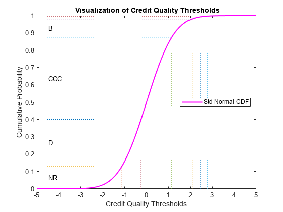
Credit quality thresholds are illustrated in the following figure. The segments in the vertical axis represent transition probabilities, and the boundaries between them determine the critical values in the horizontal axis, via the standard normal distribution. Each row in the transition matrix determines a set of thresholds. The figure shows the thresholds for the 'CCC' rating.

xliml = -5;
xlimr = 5;
step = 0.1;
x = xliml:step:xlimr;
thresCCC = thresholdMat(7,:);
centersY = (normcdf([thresCCC(2:end) xliml])+...
   normcdf([xlimr thresCCC(2:end)]))/2;
labels = {'AAA','AA','A','BBB','BB','B','CCC','D','NR'};

figure
plot(x,normcdf(x),'m','LineWidth',1.5)
for i=2:length(labels)
   val = thresCCC(i);
   line([val val],[0 normcdf(val)],'LineStyle',':');
   line([x(1) val],[normcdf(val) normcdf(val)],'LineStyle',':');
   if (centersY(i-1)-centersY(i))>0.05
      text(-4.5,centersY(i),labels{i});
   end
end
xlabel('Credit Quality Thresholds')
ylabel('Cumulative Probability')
title('{\bf Visualization of Credit Quality Thresholds}')
legend('Std Normal CDF','Location','E')

Figure contains an axes object. The axes object with title blank Visualization blank of blank Credit blank Quality blank Thresholds, xlabel Credit Quality Thresholds, ylabel Cumulative Probability contains 21 objects of type line, text. This object represents Std Normal CDF.

Shifting the critical values to the right or left changes the transition probabilities. For example, here is the transition matrix obtained by shifting the TTC thresholds by 0.5 to the right. Note that default probabilities increase.

shiftedThresholds = thresholdMat+0.5;
Example_DisplayTransitions(transprobfromthresholds(shiftedThresholds),...
   [],{'AAA','AA','A','BBB','BB','B','CCC'},...
   {'AAA','AA','A','BBB','BB','B','CCC','D','NR'})

          AAA     AA      A    BBB     BB      B    CCC      D     NR 
   AAA  75.34  13.84   1.05   0.19   0.13      0      0      0   9.45 
    AA   0.13  74.49  13.53   1.21   0.12   0.22   0.04   0.02  10.24 
     A   0.01   0.51   76.4  10.02   0.83   0.31   0.06   0.08  11.77 
   BBB      0   0.03    1.2  74.03   7.22   1.39   0.32   0.51  15.29 
    BB      0   0.01   0.05   1.77  63.35  10.94   1.47   1.88  20.52 
     B      0   0.01   0.04   0.07   1.91  59.67   5.74    8.1  24.46 
   CCC      0      0   0.05    0.1   0.36   4.61  35.06  33.18  26.65

Given a particular PIT matrix, the idea in [6] and [8] is to vary the shifting parameter applied to the TTC thresholds so that the resulting transition matrix is as close as possible to the PIT matrix. Closeness is measured as the sum of squares of differences between corresponding transition probabilities. The optimal shifting value is called credit index. A credit index is determined for every PIT transition matrix in the sample.

Here we use fminunc from Optimization Toolbox™ to find the credit indices.

CreditIndex = zeros(nYears,1);
ExitFlag = zeros(nYears,1);
options = optimset('LargeScale','Off','Display','Off');
for i=1:nYears
   errorfun = @(z)norm(squeeze(TransMat(:,:,i))-...
      transprobfromthresholds(...
      transprobtothresholds(tmTTC)+z),'fro');
   [CreditIndex(i),~,ExitFlag(i)] = fminunc(errorfun,0,options);
end

In general, one expects that higher credit indices correspond to riskier years. The series of credit indices found does not entirely match this pattern. There may be different reasons for this. First, transition probabilities may deviate from their long-term averages in different ways that may lead to confounding effects in the single parameter trying to capture these differences, the credit index. Having separate credit indices for IG and SG, for example, may help separate confounding effects. Second, a difference of five basis points may be very significant for the 'BBB' default rate, but not as important for the 'CCC' default rate, yet the norm used weights them equally. Other norms can be considered. Also, it is always a good idea to check the exit flags of optimization solvers, in case the algorithm could not find a solution. Here we get valid solutions for each year (all exit flags are 1).

figure
plot(Years,CreditIndex,'-d')
hold on
Example_RecessionBands
hold off
grid on
xlabel('Year')
ylabel('Shift')
title('{\bf Credit Index}')

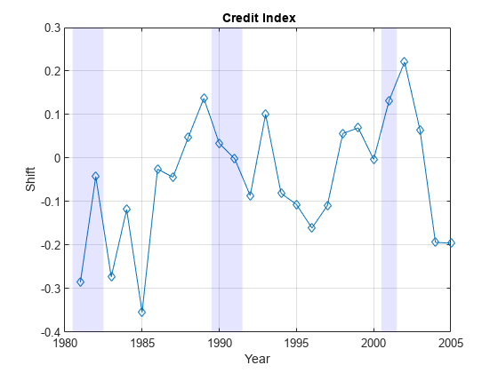
Figure contains an axes object. The axes object with title blank Credit blank Index, xlabel Year, ylabel Shift contains 6 objects of type line, patch.

The workflow above can be adapted to work with the series of credit indices instead of the series of corporate default rates. A model can be fit to predict a credit index for the following year, and a predicted transition matrix can be inferred and used for risk analyses.

References

[1] Altman, E., and E. Hotchkiss, Corporate Financial Distress and Bankruptcy, third edition, New Jersey: Wiley Finance, 2006.

[2] Basel Committee on Banking Supervision, "International Convergence of Capital Measurement and Capital Standards: A Revised Framework," Bank for International Settlements (BIS), comprehensive version, June 2006. Available at: https://www.bis.org/publ/bcbsca.htm.

[3] Basel Committee on Banking Supervision, "Principles for Sound Stress Testing Practices and Supervision - Final Paper," Bank for International Settlements (BIS), May 2009. Available at: https://www.bis.org/publ/bcbs155.htm.

[4] FRED, St. Louis Federal Reserve, Federal Reserve Economic Database, https://fred.stlouisfed.org/.

[5] Helwege, J., and P. Kleiman, "Understanding Aggregate Default Rates of High Yield Bonds," Federal Reserve Bank of New York, Current Issues in Economics and Finance, Volume 2, Number 6, May 1996.

[6] Loeffler, G., and P. N. Posch, Credit Risk Modeling Using Excel and VBA, West Sussex, England: Wiley Finance, 2007.

[7] NBER, National Bureau of Economic Research, Business Cycle Expansions and Contractions, https://www.nber.org/research/business-cycle-dating.

[8] Otani, A., S. Shiratsuka, R. Tsurui, and T. Yamada, "Macro Stress-Testing on the Loan Portfolio of Japanese Banks," Bank of Japan Working Paper Series No.09-E-1, March 2009.

[9] Survey of Professional Forecasters, Federal Reserve Bank of Philadelphia, https://www.philadelphiafed.org/.

[10] Vazza, D., D. Aurora, and R. Schneck, "Annual 2005 Global Corporate Default Study And Rating Transitions," Standard & Poor's, Global Fixed Income Research, New York, January 2006.

[11] Wilson, T. C., "Portfolio Credit Risk," FRBNY Economic Policy Review, October 1998.