Track-Level Fusion of Radar and Lidar Data in Simulink
Autonomous systems require precise estimation of their surroundings to support decision making, planning, and control. High-resolution sensors such as radar and lidar are frequently used in autonomous systems to assist in estimation of the surroundings. These sensors generally output tracks. Outputting tracks instead of detections and fusing the tracks together in a decentralized manner provide several benefits, including low false alarm rates, higher target estimation accuracy, a low bandwidth requirement, and low computational costs. This example shows you how to track objects from measurements of a radar and a lidar sensor and how to fuse them using a track-level fusion scheme in Simulink®. You process the radar measurements using a Gaussian Mixture Probability Hypothesis Density (GM-PHD) tracker and the lidar measurements using a Joint Probabilistic Data Association (JPDA) tracker. You further fuse these tracks using a track-level fusion scheme. The example closely follows the Track-Level Fusion of Radar and Lidar Data MATLAB® example.
Overview of Model
load_system('TrackLevelFusionOfRadarAndLidarDataInSimulink');
set_param('TrackLevelFusionOfRadarAndLidarDataInSimulink','SimulationCommand','update');
open_system('TrackLevelFusionOfRadarAndLidarDataInSimulink');
The model has six subsystems, each implementing a part of the algorithm.
Scenario and Sensor Simulation
Radar Tracking Algorithm
Lidar Tracking Algorithm
Track Level Fusion
Performance Analysis
Visualization
Scenario and Sensor Simulation
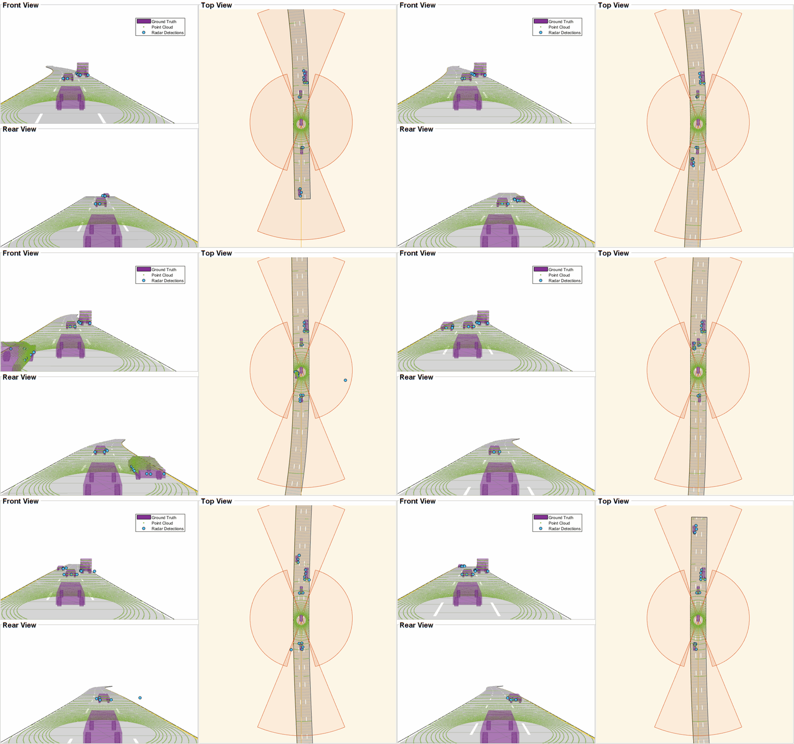
The scenario recording for this example is captured from the scenario described in Track-Level Fusion of Radar and Lidar Data MATLAB example. The Scenario Reader block reads a prerecorded scenario file and generates actors and ego vehicle position data as Simulink.Bus (Simulink) objects. In this scenario, the ego vehicle is mounted with four 2-D radar sensors. The front and rear radar sensors have a field of view of 45 degrees. The left and right radar sensors have a field of view of 150 degrees. Each radar has a resolution of 6 degrees in azimuth and 2.5 meters in range. The ego vehicle is also mounted with one 3-D lidar sensor with a field of view of 360 degrees in azimuth and 40 degrees in elevation. The lidar has a resolution of 0.2 degrees in azimuth and 1.25 degrees in elevation (32 elevation channels). The Radar Detection Generator block generates radar detections and the Lidar Point Cloud Generator block generates point clouds. Detections from all four radar sensors are grouped together with the Detection Concatenation block and the Digital Clock block is used to simulate time. Sensor configurations and the simulated sensor data is visualized in the animation that follows. Notice that the radars have higher resolution than objects and therefore return multiple measurements per object. Also notice that the lidar interacts with the actors as well as the road surface to return multiple points.


Radar Tracking Algorithm
Radars generally have higher resolution than the objects and return multiple detections per object. Conventional trackers such as Global Nearest Neighbor (GNN) and Joint Probabilistic Data Association (JPDA) assume that the sensors return at most one detection per object per scan. Therefore, the detections from high-resolution sensors must be either clustered before processing them with conventional trackers or must be processed using extended object trackers. Extended object trackers do not require preclustering of detections. Generally, extended object trackers offer better estimation of objects since they handle clustering and data association simultaneously.
In this example, you use a Gaussian mixture probability hypothesis density (GM-PHD) extended object tracker for radar tracking. The tracker block takes detections, prediction time, and sensor configurations as input and outputs confirmed tracks as a Simulink.Bus (Simulink) object. Detections from the radar are preprocessed to include ego vehicle INS information in the Radar Detection Preprocessing MATLAB Function (Simulink) Block. The Sensor Configuration Reader block provides Sensor Configuration to the tracker block. The block is implemented by using MATLAB System (Simulink) block. Code for this block is defined in the HelperSourceConfigReader class.
This visualization shows radar tracking at a single time step. Notice that the radar sensors report multiple detections per object and the GM-PHD tracker forms two-dimensional rectangular tracks corresponding to each object.
![]()
Lidar Tracking Algorithm
Lidar sensors have high resolution capabilities, and each scan from the sensor contains many points, commonly known as a point cloud. This raw data must be preprocessed to extract objects. The preprocessing is performed using a RANSAC-based plane-fitting algorithm and bounding boxes are fitted using a Euclidian-based distance clustering algorithm. For more information about the algorithm, refer to the Track Vehicles Using Lidar: From Point Cloud to Track List example.
The Bounding Box Detector block is implemented using a MATLAB System (Simulink) block. Code for this block is defined in a helper class, HelperBoundingBoxDetectorBlk. The block accepts point cloud locations and a prediction time as input and outputs bounding box detections corresponding to obstacles and segmentation information. Detections are processed using a conventional JPDA tracker, configured with an interacting multiple model (IMM) filter. The IMM filter is implemented using the helper function helperInitIMMUKFFilter, which is specified as the Filter initialization function parameter of the block. Detections from lidar sensor are preprocessed to include ego vehicle INS information in the Lidar Detection Preprocessing MATLAB Function (Simulink) block.
The Calculate Detectability block calculates the Detectable TrackIDs input for the tracker and outputs an two-column array. The first column represents the TrackIDs of the tracks and the second column specifies their detection probability by the sensor and bounding box detector. The block is implemented using a MATLAB Function (Simulink) block.
This visualization shows the lidar tracking at a single time step. The Bounding Box Detector block generates detections from the point cloud, and the JPDA tracker forms three-dimensional cuboid tracks corresponding to each object.
![]()
Track-Level Fusion
The track fusion algorithm is implemented using the Track-To-Track Fuser block. The block takes a prediction time, rectangular radar tracks, and cuboid lidar tracks as input and outputs fused tracks. It uses a traditional track-to-track association-based fusion scheme and GNN assignment to create a single hypothesis. The Track Concatenation block combines tracks from both sources and generates a single track bus. The fuser source configuration for radar and lidar is set using the SourceConfig variable through the PreLoadFcn callback. See Model Callbacks (Simulink) for more information about callback functions. The state fusion algorithm for this example is implemented in the helperRadarLidarFusionFunction helper function and specified as the 'custom fusion function' property.
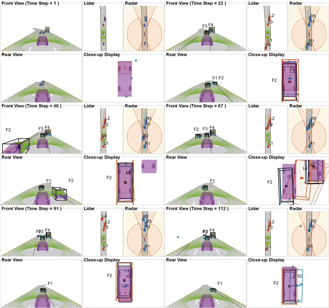
This visualization shows track fusion at a single time step. The fused tracks are closer to the actual objects than the individual sensor tracks, which indicates that track accuracy increased after fusion of track estimates from both sensors.

Performance Analysis
In this example, you assess the performance of each algorithm using the Generalized Optimal Subpattern Assignment (GOSPA) metric. The GOSPA metric aims to evaluate the performance of a tracking system with a scalar cost.
The GOSPA metric can be calculated with the following equation
![$GOSPA = [\sum_{i=0}^{m}(min(d_{b},c))^{p} + \frac{c^{p}}{\alpha} (n-m)]^{1/p}$](../../examples/shared_driving_fusion_lidar/win64/TrackLevelFusionOfRadarAndLidarDataInSimulinkExample_eq08558369401179169166.png)
where  is the number of ground truths,
  is the number of estimated tracks,
  is the cutoff distance threshold,
  is the base distance between track and truth calculated by a distance function specified in the
 Distance property,  is order of the metric and
  is the alpha parameter of the metric, defined from the block mask.
A lower value of the metric indicates better performance of the tracking algorithm. To use the GOSPA metric with custom motion models like the one used in this example, you set the Distance property to custom and define a distance function between a track and its associated ground truth. These distance functions are defined in helperRadarDistance and helperLidarDistance helper files. The Ground Truth Reader block provides truth data at each time step. The block is implemented using a MATLAB System (Simulink) block and code for this block is defined in the HelperGroundTruthReader class. Finally, the GOSPA score for radar tracking, lidar tracking, and track fusion algorithms are grouped together.
Visualization
The Visualization block is implemented using a MATLAB System (Simulink) block. Code for this block is defined in the helper class helperLidarRadarTrackFusionDisplayBlock. The block uses the RunTimeObject parameter of the blocks to display their outputs. See Access Block Data During Simulation (Simulink) for further information on how to access block outputs during simulation.
This animation shows the entire run every three time steps. Each three tracking system (radar, lidar, and track-level fusion) was able to track all four vehicles in the scenario without confirming any false tracks.

The GOSPA metric is visualized using the scope block. The x-axis in the figure that follows represents time and y-axis represents the GOSPA score. Each unit on the x-axis represents 10 time steps in the scenario. The track-level localization accuracy of each tracker can be quantitatively assessed with the GOSPA metric at each time step. A lower value indicates better tracking accuracy. As there were no missed targets or false tracks, the metric captures the localization errors resulting from the state estimation of each vehicle. Each component of the GOSPA metric can also be selected as a block output and visualized separately.
Note that the GOSPA metric for fused estimates is lower than the metric for individual sensor, which indicates that track accuracy increased after fusion of track estimates from both sensors.
close_system('TrackLevelFusionOfRadarAndLidarDataInSimulink');
Summary
In this example, you learned how to track radar measurements using an extended object tracker with a two-dimensional rectangular model, how to track lidar measurements using a conventional JPDA tracker with a three-dimensional cuboid model, and how to set up a track-level fusion algorithm for fusing tracks from radar and lidar sensors in Simulink. You also learned how to evaluate performance of a tracking algorithm using the Generalized Optimal Subpattern Assignment metric. The simulation results show that tracking by fusing tracks from radar and lidar is more accurate than tracking by each individual sensor.