Model a Thermal Liquid Pipeline

This tutorial shows how to model a pump-driven thermal liquid pipeline. The pipeline system comprises a pump, a pipe, and two thermal liquid reservoirs. The pump generates power and the pipe transfers fluid between the reservoirs. The reservoirs act as pressure and temperature boundary conditions for the pipeline system. Note that "thermal" refers to the properties of the solid system, while "thermal liquid" refers to the properties of the fluid system.

Thermal Liquid Pipeline Schematic

The reservoir conditions are fixed at room temperature, 293.15 K, and atmospheric pressure, 0.101325 MPa. The outer pipe surface temperature is fixed at a temperature of 275 K. The pipe fluid volume is initially at room temperature but, through the combined effects of heating due to friction and conductive cooling, gradually shifts toward a new steady-state value. The thermal resistance of the pipe is the combination of these convective and conductive resistances.

Pipe Thermal Resistances

Composite of thermal resistances in wall

A Pipe (TL) block models the convective thermal resistance at the inner pipe surface and the heating due to friction in the thermal liquid. A Conductive Heat Transfer block models the conductive thermal resistance between the inner and outer pipe surfaces.

Start a New Model

At the MATLAB^® command prompt, enter sscnew. MATLAB opens the Simscape™ model template. This template provides a starting point for your Simscape Fluids™ model, and includes a Solver Configuration block, a Simulink-PS converter block, a PS-Simulink converter block, and a Scope block, which enables you to view the results of your simulation. You will not need the Simulink-PS Converter block in this example.
Save the model often as you add new blocks.
In the Simulation tab, click Library Browser. In the pop-up window, select Simscape > Foundation Library > Thermal Liquid > Utilities library and drag a Thermal Liquid Settings (TL) block to the model canvas. This block defines the physical properties of the thermal liquid, including its viscosity, thermal conductivity, and bulk modulus.
Connect the Solver Configuration and Thermal Liquid Settings (TL) blocks as shown in the figure. The Solver Configuration block provides Simscape solver settings for your model. Each physical network requires a Solver Configuration block.

Model the Pipeline

Open the Library Browser. Select Simscape > Foundation Library > Thermal Liquid > Elements library, drag two Reservoir (TL) blocks to the model canvas. The reservoir blocks set the pressure and temperature boundary conditions for the pipeline model.

From the Simscape > Fluids > Thermal Liquid library, insert these blocks.

Block	Library	Purpose
Pipe (TL)	Pipes & Fittings	Conduit for thermal liquid between reservoirs
Fixed-Displacement Pump (TL)	Pumps & Motors	Power generation source

Connect the blocks and verify your connections in the figure below. Note that blocks may be rotated.
1. Port A of the Pipe (TL) block connects to port B of the Fixed-Displacement Pump (TL) block.
2. Port B of the Pipe (TL) block connects to one Reservoir (TL) block. This serves as a thermal liquid sink.
3. Port A of the Fixed-Displacement Pump (TL) block connects to the second Reservoir (TL) block, the Solver Configuration block, and the Thermal Liquid Settings (TL) block. The Reservoir block serves as a thermal liquid source.
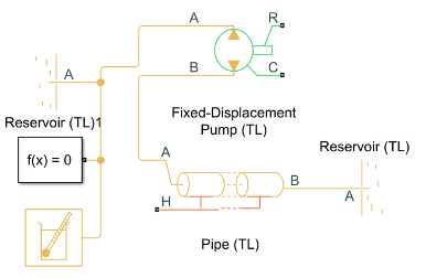
The component colors indicate the physical domains they represent: yellow for Thermal Liquid, red for Thermal, and green for Mechanical Rotational. The pump and pipe blocks are multi-domain blocks that you can use to interface different physical domains.
In the Pipe (TL) block, set the Pipe length parameter to 1000 m. This length results in observable pressure losses due to dissipation and heat transfer by friction at the pipe walls.

Introduce Thermal Conduction

Open the Library Browser and insert these blocks from the Simscape > Foundation Library.

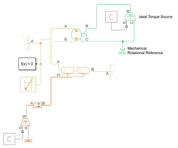
Block	Library	Purpose
Conductive Heat Transfer	Thermal > Thermal Elements	Models the conductive heat losses through the pipe wall to the surrounding environment
Thermal Reference	Thermal > Thermal Elements	Provides a temperature reference for the physical signal input
Controlled Temperature Source	Thermal > Thermal Sources	Acts as an ideal energy source and maintains temperature regardless of heat flow rate
PS Constant	Physical Signals > Sources	Specifies environmental temperature

Connect the blocks and verify your connections in the figure below. Note that blocks may be rotated.
1. Connect port B of the Conductive Heat Transfer block to port H of the Pipe (TL) block.
2. Connect port B of the Controlled Temperature Source block to port A of the Conductive Heat Transfer block.
3. Connect the PS Constant block to port S of the Controlled Temperature Source block.
4. Connect the Thermal Reference block to port A of the Controlled Temperature Source block.
In the PS Constant Block Parameters Window, set the Constant parameter to 275 K. This is the environment temperature.
In the Conductive Heat Transfer block, set the Area parameter to pi*0.1128*1000 m ². This is the pipe surface area in terms of the hydraulic diameter, 0.1128 m, and length, 1000 m. The default Thermal conductivity value is for copper, 401 W/(mK)].

Model the Pump Torque

Open the Library Browser and insert these blocks from SimscapeFoundation Library.

Block	Library	Purpose
Ideal Torque Source	Mechanical > Mechanical Sources	Sets the pump torque rate as a physical signal
Mechanical Rotational Reference	Mechanical > Rotational Elements	Acts as a reference for the Ideal Torque Source and maintains a physical signal at a specified value
PS Constant	Double-click on the browser white space, type PS Constant and hit Enter	Specifies the pump torque

Connect the blocks and verify your connections in the figure. Note that blocks may be rotated.
1. Connect port R of the Fixed-displacement Pump (TL) block, which represents the rotating pump shaft, to port R of the Ideal Torque Source block.
2. Connect port C of the Ideal Torque Source block, which represents pump casing, to port C of the Fixed-Displacement Pump (TL) block and the Mechanical Rotational Reference block.
3. Connect port S of the Ideal Torque Source block to the PS Constant block.
In the PS Constant Block Parameters window, set the Constant parameter to 50 N*m.

Add Thermal Liquid Sensors

Open the Library Browser and add these blocks to the model.

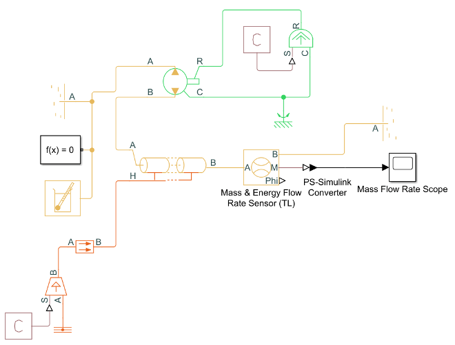
Block	Library	Purpose
Flow Rate Sensor (TL)	Simscape > Foundation Library > Thermal Liquid > Sensors	Measures the Through variables of the Thermal Liquid domain and returns a physical signal
PS-Simulink Converter	Simscape > Utilities	Transforms a physical signal into a Simulink^® signal
Scope	Simulink > Sinks	Plots Simulink signals

Connect the blocks and verify your connections in the figure. Note that blocks may be rotated.
1. Your Pipe (TL) block is connected to a Reservoir from Section 1.5.4, which provides pressure and temperature boundary conditions for the system. You will now add a way to measure pipe flow. Disconnect port B of the Pipe (TL) block from the Reservoir block and connect it to port A of the Mass & Energy Flow Rate Sensor (TL) block.
2. Connect port B of the Mass & Energy Flow Rate Sensor block to the Reservoir block.
3. Connect port M of the Mass & Energy flow Rate Sensor (TL) block to the PS-Simulink Converter block.
4. Connect the PS-Simulink Converter block to the Scope block. Click the Scope block and name it "Mass Flow Rate Scope."

Open the Library Browser and add these blocks to the model. You will also use the PS-Simulink Converter and Scope blocks that were included when you opened your new model.

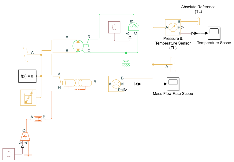
Block	Library	Purpose
Pressure & Temperature Sensor (TL)	Simscape > Foundation Library > Thermal Liquid > Sensors	Measures the Across variables of the Thermal Liquid domain and returns a physical signal
Absolute Reference (TL)	Simscape > Foundation Library > Thermal Liquid > Elements	Provides a control reference where pressure and temperature are equal to zero

Connect the blocks and verify your connections in the figure. Note that blocks may be rotated.
1. Create a branch from port B of the Mass & Energy Flow Rate Sensor (TL) block and connect it to port A of the Pressure & Temperature Sensor (TL) block.
2. Connect port B of the Pressure & Temperature Sensor(TL) block to the Absolute Reference block.
3. Connect port T of the Pressure & Temperature Sensor (TL) block to the PS-Simulink Converter block.
4. If the PS-Simulink Converter is not already connected to the remaining Scope block, connect the two. Click this Scope block and name it "Temperature Scope."

Simulate the Pipeline Model

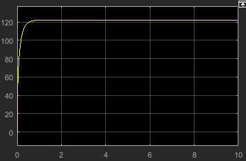
The Simscape model template specifies suitable solver settings for this model. You can run the simulation by opening the Simulation tab and clicking Run > Run. Once the model has compiled, open the Mass Flow Rate Scope. Your plot should show a quick change in flow rate as the thermal liquid transitions from a state of rest to a new steady-state velocity.

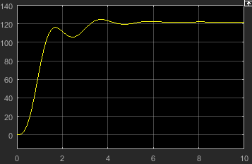
You can experiment with other block settings and input signals. Try setting the Pipe (TL) block Fluid inertia parameter to On, then run your model. The figure shows the combined effects of fluid dynamic compressibility and fluid inertia on the mass flow rate plot.