Analyze Optical System Using Optical System Designer

This example uses:

Image Processing Toolbox Image Processing Toolbox
Optical Design and Simulation Library for Image Processing Toolbox Optical Design and Simulation Library for Image Processing Toolbox

This example shows how to analyze an optical system using the Optical System Designer app. The Optical System Designer app enables you to design, modify, simulate, and analyze optical systems. Using the app, you can:

Create a new optical system or load an existing optical system from a ZMX file or the MATLAB® workspace.
Visualize the optical system in 2-D or 3-D.
Design a new optical system using various components, materials, and light sources, or modify an existing optical system.
Simulate ray tracing, and focus the optical system.
Analyze the optical system using spot diagrams, ray and chromatic aberration analysis, lens distortion analysis, and field curvature analysis.
Export the designed optical system as an opticalSystem object to the workspace or as a function you can use to create similar optical systems.

For information on how to design an optical system using the app, see Design Optical System Using Optical System Designer.

Open the Optical System Designer App

Open the Optical System Designer app from the Apps tab on the MATLAB Toolstrip, under Image Processing and Computer Vision, by selecting the Optical System Designer icon. You can also open the app by using the opticalSystemDesigner command at the MATLAB command prompt.

Load Optical System

To import an existing optical system, select Import on the Optical System tab of the app toolstrip. Then select one of these options.

To import an optical system from a ZMX file, select From ZMX File. Then, in the dialog box, select your ZMX file.
To import an optical system from the workspace, select From Workspace. Then, in the dialog box, select your opticalSystem object.

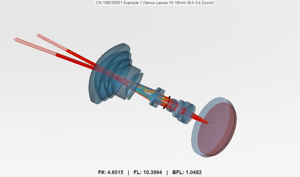
Import the optical system from PhotographicLens.zmx file attached to this example as a supporting file.

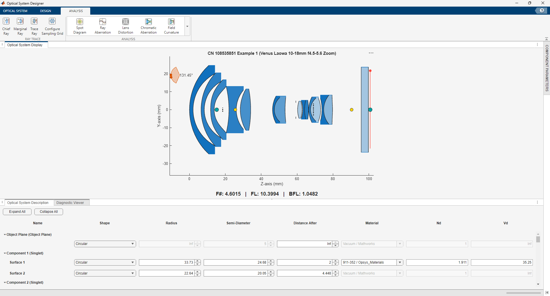
Optical system of photographic lens loaded from ZMX file into Optical System Designer app.

Alternatively, to create a new optical system, on the Optical System tab, select New to open an empty canvas to which you can add optical elements.

Trace Rays

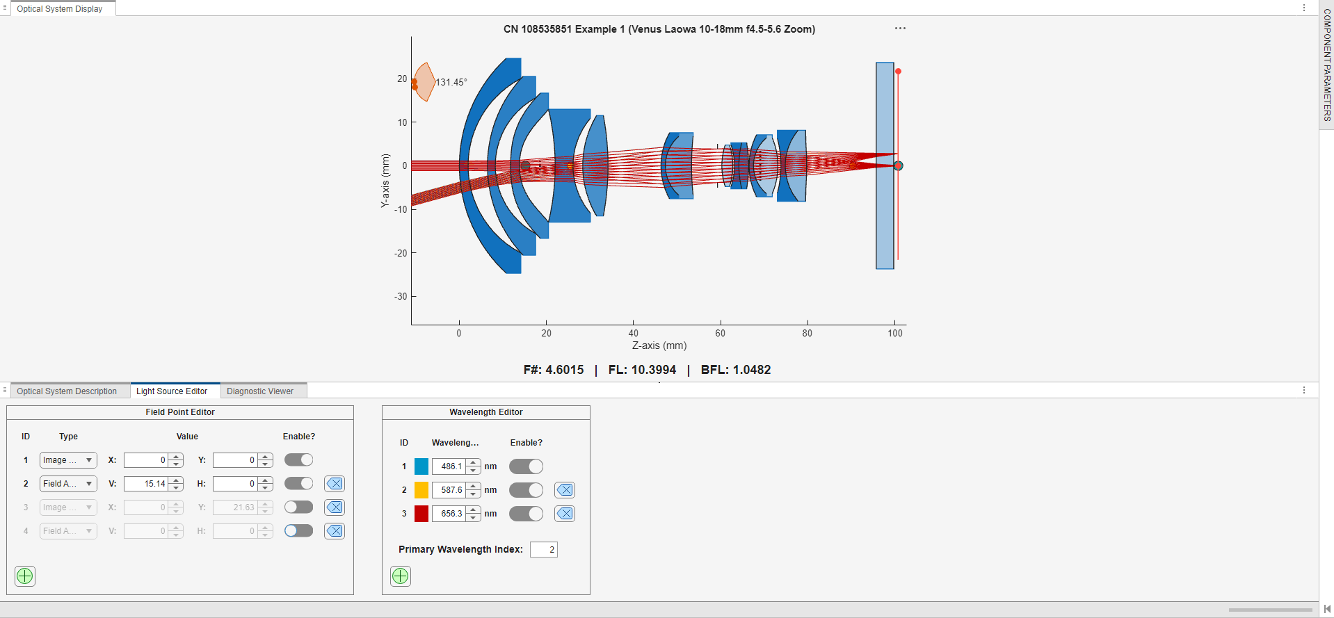
This example analyzes the optical system using only two field points and three wavelengths. Enable the Light Source Editor on the Optical System tab of the app toolstrip, by selecting Light Source. In the Field Point Editor section of the Light Source Editor pane, turn off field points 3 and 4 by selecting the corresponding toggles in the Enable? column.

On the Analysis tab of the app toolstrip, you can select Chief Ray to trace chief rays, Marginal Ray to trace marginal rays, or Trace Ray to trace all rays. Select Trace Ray, and observe from the ray tracing that the optical system is focused, as the rays converge at the focal point on the image plane.

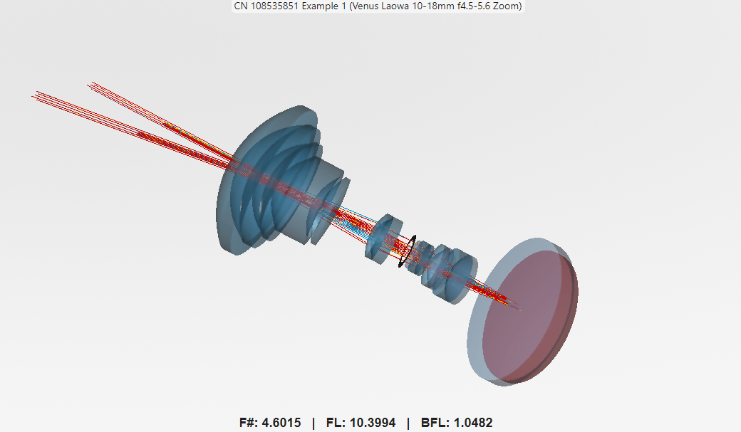
Ray tracing for optical system in Optical System Designer app.

Visualize the optical system in 3-D by selecting the 3-D option in the View section of the Optical System tab. You can rotate and zoom the 3-D view for better visualization.

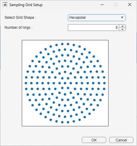
3-D visualization of optical system in Optical System Designer app.

You can also specify the shape of the sampling grid by selecting Configure Sampling Grid and, in the Sampling Grid Setup dialog box, setting Select Grid Shape to Square, Hexapolar, Random, or Default. You can additionally specify the number of points per side for a square grid, the number of rings for a hexapolar grid, and the number of points for a random grid. Return to the 2-D visualization after configuring the sampling grid.

Sampling Grid Setup in Optical System Designer app.

3-D visualization of optical system with hexapolar sampling grid in Optical System Designer app.

Analyze Optical System

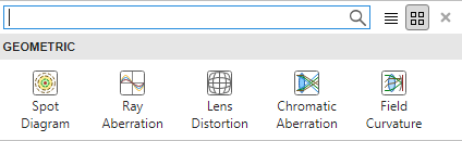
You can perform these analyses on your optical system, to assess how well it forms an image, by selecting them from the Analysis section of the Analysis tab of the app toolstrip.

Spot Diagrams — Shows how tightly light rays focus.
Ray Aberration — Reveals deviations from the ideal path.
Lens Distortion — Assesses the shape accuracy of the image.
Chromatic Aberration — Assesses the color accuracy of the image.
Field Curvature — Assesses if the image stays sharp across the entire field.

Analysis gallery in Optical System Designer app.

Spot Diagram

A spot diagram shows how light rays from a single point on an object focus after passing through an optical system. Ideally, all rays should meet at one point. However, due to imperfections, they spread out into a small cluster called a spot. This analysis helps visualize image sharpness.

To generate the spot diagrams, select Spot Diagram in the Analysis section of the Analysis tab. The app opens the Spot Diagram pane, with spot diagrams for each field point.

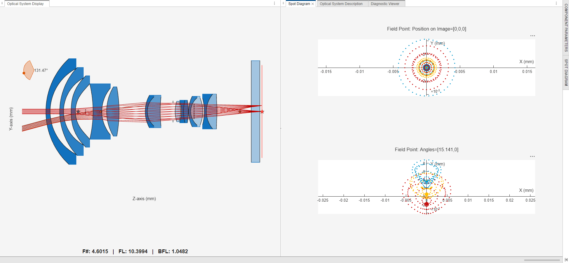
Spot diagram analysis for optical system in Optical System Designer app.

The spot diagram for each field point shows a cluster of dots representing where rays from a single object point land on the image plane. If the dots are tightly packed and close to the center, the system has good focus and minimal aberrations. Larger or spread-out clusters indicate blur or optical errors.

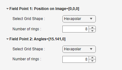
To modify the grid shape and number of rings for each field point, select Spot Diagram on the right side of the app window. For more information about spot diagram analysis, see the spot function.

Spot Diagram options on the right side of the app window.

Ray Aberration

Ray aberration measures how far individual rays deviate from their ideal position at the image plane. Instead of forming a perfect image point, rays land at slightly different locations because of lens imperfections. This analysis helps identify deviations from the ideal path.

To generate the ray aberration plots, select Ray Aberration in the Analysis section of the Analysis tab. The app opens the Ray Aberration pane, with plots for the tangential and sagittal orientation of each field point.

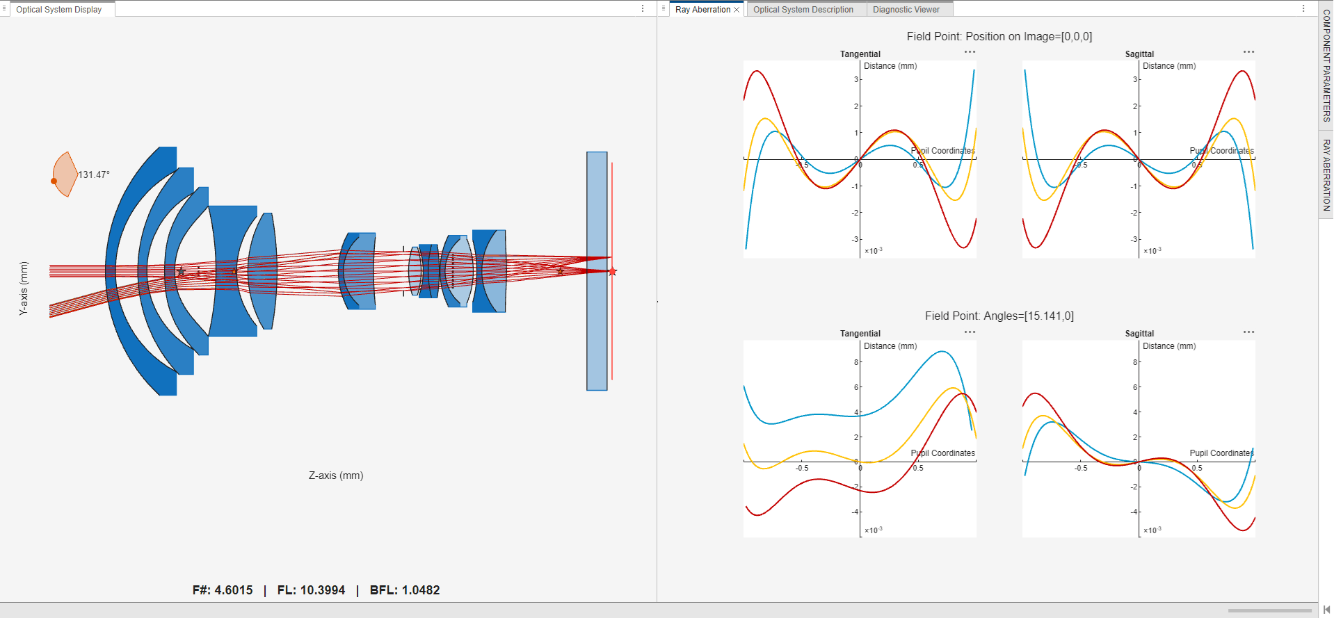
Ray aberration analysis for optical system in Optical System Designer app.

The ray aberration plots show the deviation of each ray from the ideal image point against the position of the entrance pupil. Each field point has one plot for tangential rays and one for sagittal rays. Tangential rays lie in the plane that contains the optical axis and the chief ray for that field point. Sagittal rays lie in the plane perpendicular to the tangential plane. Ideally, the deviations in the plot are close to zero. Large deviations or steep slopes indicate aberrations. Symmetry in curves often indicates balanced design, whereas asymmetry suggests misalignment or design flaws.

To modify the number of samples for each field point, select Ray Aberration on the right side of the app window. For more information about ray aberration analysis, see the rayAberration function.

Ray Aberration options on the right side of the app window.

Lens Distortion

Lens distortion changes the shape of the image compared to the subject of the image. Straight lines might appear curved, and objects might appear stretched or compressed. This analysis helps assess shape accuracy.

To generate the lens distortion diagram, select Lens Distortion in the Analysis section of the Analysis tab. The app opens the Lens Distortion pane, with the lens distortion diagram.

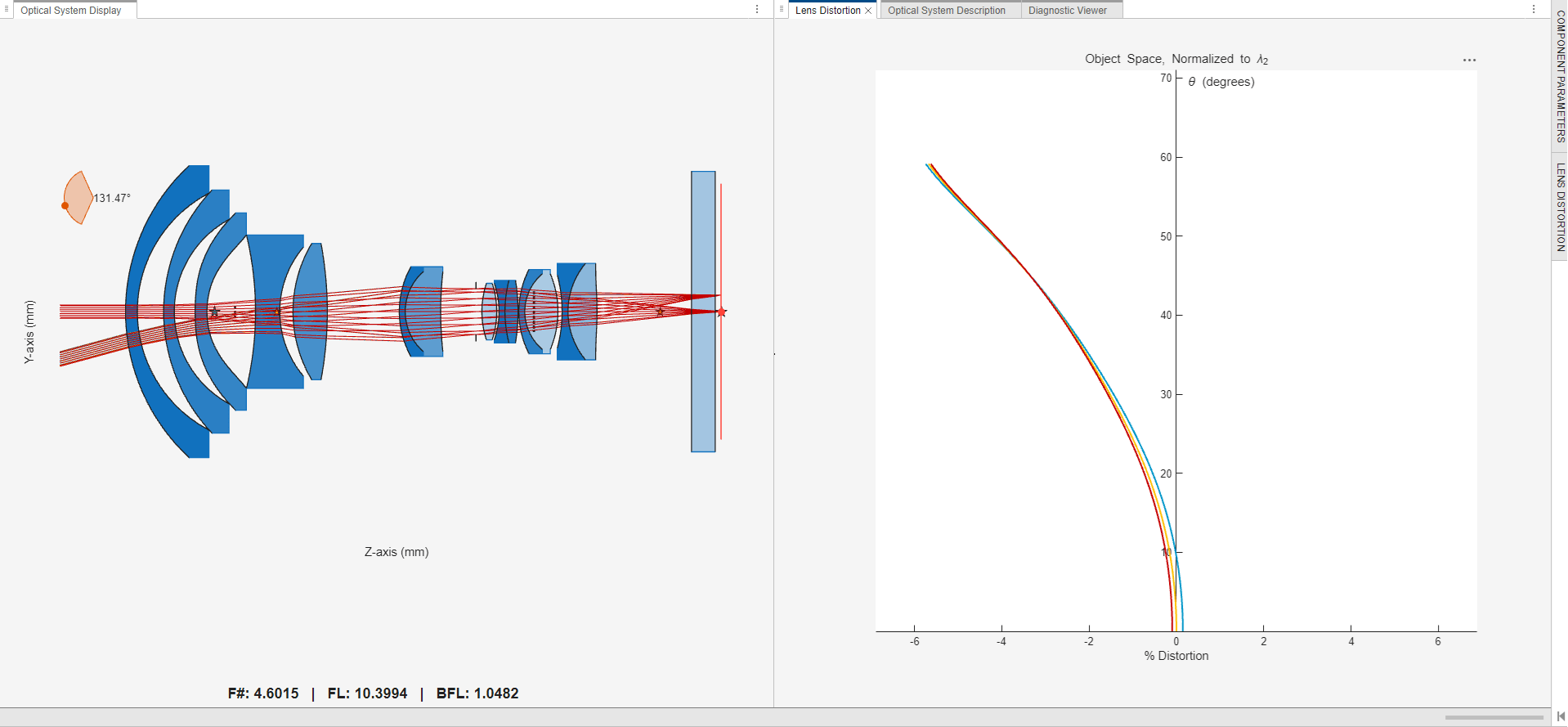
Lens distortion analysis for optical system in Optical System Designer app.

The lens distortion diagram shows a plot of the field angle against the percentage distortion. A vertical line near 0% indicates minimal distortion across the field, while a curve indicates distortion.

To modify the scale, maximum field angle, distortion type, computation space, and number of samples, select Lens Distortion on the right side of the app window. For more information about lens distortion analysis, see the lensDistortion function.

Lens Distortion options on the right side of the app window.

Chromatic Aberration

Chromatic aberration occurs because lenses bend different wavelengths by different amounts. As a result, all colors do not focus at the same point, creating color fringes around objects. This analysis helps assess how much color separation occurs, enabling you to design lenses or coatings to minimize it.

To generate the chromatic aberration plots, select Chromatic Aberration in the Analysis section of the Analysis tab. The app opens the Chromatic Aberration pane, with plots for lateral and longitudinal aberration.

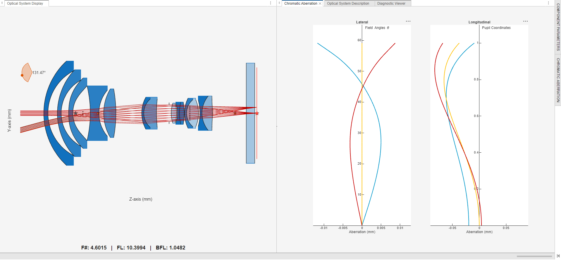
Chromatic aberration analysis for optical system in Optical System Designer app.

The lateral aberration plot shows the field angle against the aberration. If the curves for different wavelengths stay near zero across all field angles, lateral chromatic aberration is well corrected. Larger shifts at higher field angles indicate more color fringing toward the edges. The longitudinal aberration plot shows the pupil coordinates against the aberration. If curves for different wavelengths overlap near zero and focus at the same point, longitudinal chromatic aberration is corrected. A spread between the curves for different wavelengths indicates that different colors focus at different depths, causing blur and color halos.

To modify the maximum field angle and number of samples select Chromatic Aberration on the right side of the app window. For more information about chromatic aberration analysis, see the chromaticAberration function.

Chromatic Aberration options on the right side of the app window.

Field Curvature

Field curvature indicates that the image plane is not perfectly flat. If the center of the image is in focus, the edges might be blurry, or the other way round. This analysis shows how much the focus shifts across the field, and helps you correct designs for flat sensors or screens.

To generate the field curvature plots, select Field Curvature in the Analysis section of the Analysis tab. The app opens the Field Curvature pane, with plots for tangential and sagittal rays.

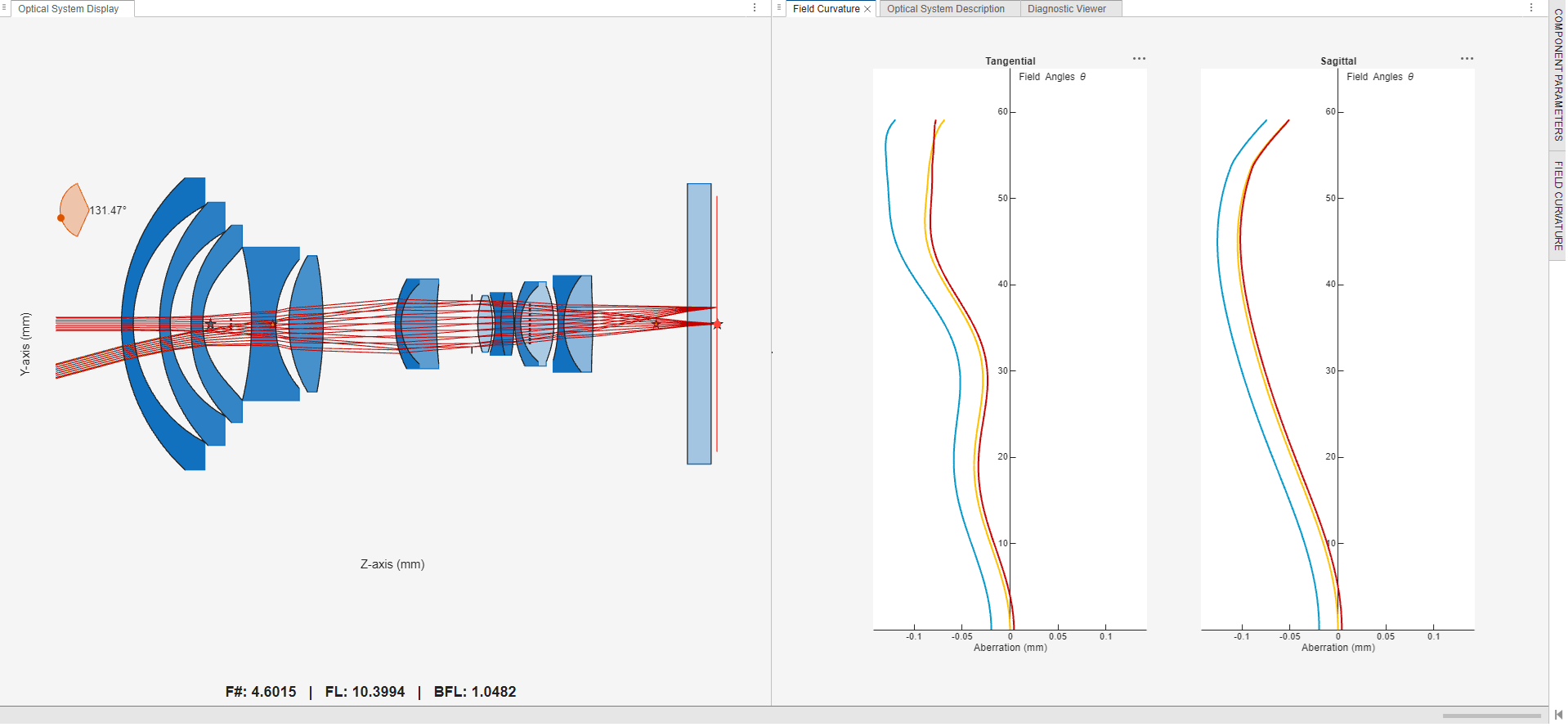
Field curvature analysis for optical system in Optical System Designer app.

The field curvature plots show the field angles against the aberration. If both curves have near zero aberration across field angles, you can consider the image plane to be flat. If curves bend away from zero, the image surface is curved. Separation between the tangential and sagittal curves indicates differences in focus for the two planes. Larger curvature indicates more blur at the edges when the center is in focus.

To modify the maximum field angle and number of samples select Field Curvature on the right side of the app window. For more information about field curvature analysis, see the fieldCurvature function.

Field Curvature options on the right side of the app window.