chromaticAberration
Compute lateral and longitudinal chromatic aberration of optical system
Since R2026a
Description
Add-On Required: This feature requires the Optical Design and Simulation Library for Image Processing Toolbox add-on.
ca = chromaticAberration(opsys,Name=Value)NumSamples=200 specifies to compute the
chromatic aberration at 200 evenly spaced coordinate points.
Examples
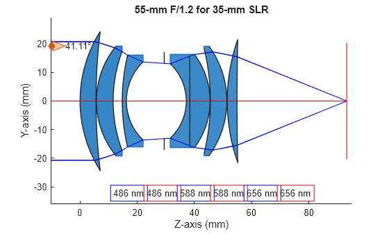
Load a double Gauss lens from a ZMX file into the workspace.
opsys = zmximport("DoubleGaussLens.zmx");Internal error: ERROR: phRayTrace::TraceSequential()- Hit wrong side of surface
Trace the marginal rays and the chief ray for the optical system.
mrays = traceMarginalRays(opsys);
cray = traceChiefRay(opsys);
Display a 2-D visualization of the optical system and the traced rays. The displayed chief ray is red, and the marginal rays are blue.
hv = view2d(opsys);
addRays(hv,mrays,Color="b")
addRays(hv,cray,Color="r")
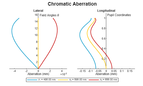
Compute the chromatic aberration of an optical system using the chromaticAberration object function. Specify the maximum field angle as 15 degrees using the MaxFieldAngle name-value argument. Display the results using the show object function.
ca = chromaticAberration(opsys,Wavelengths=[486 586 656],MaxFieldAngle=15);
show(ca)
ans =
  ChromaticAberrationChart with properties:

    ChromaticAberration: [1×1 optics.result.ChromaticAberration]
                  Color: [3×3 double]
                  Title: "Chromatic Aberration"
                 Legend: on
                   Grid: "off"
                 Parent: [1×1 Figure]

  Show all properties
Input Arguments
Name-Value Arguments
Output Arguments
More About
Algorithms
Version History
Introduced in R2026a