Model Dynamic Optical Systems with Scanning Elements
R2026bThis example shows how to model dynamic optical systems by coupling ray tracing and optical analysis with Simulink control loops. The example uses a laser etching system as a motivating application – a class of systems where mechanical motion and optical behavior are tightly coupled. You control mirror angles to steer the beam through the optical system and realize a specified etch pattern on the image plane. At each simulation timestep, ray tracing computes the resulting spot position from the current mirror angles. This closes the loop between control inputs, mechanical motion, and optical response, enabling accurate pattern tracing while revealing effects such as cross-axis coupling and showing how to correct it by using a calibration lookup table.
In this example, you construct each of the following subsystems individually and integrate them into a closed-loop simulation:
F-theta scan lens — A purely optical design that enforces a linear relationship between the incoming beam angle and the resulting spot position on the image plane. This mapping enables uniform spatial scaling and consistent scan trajectories across the field.
Dual-axis galvanometer (galvo) mirrors — Two independently driven mirrors steer the beam by dynamically varying its angle of incidence. The upstream mirror, Galvo X, tilts about the Y-axis to control the X-spot position, while the downstream mirror, Galvo Y, tilts about the X-axis to control the Y-spot position. Because Galvo Y is downstream, its effect on the image plane depends on the current Galvo X angle, creating cross-axis coupling on the Y-spot position.
Input laser beam — The source of optical energy used for etching. Detailed modeling of the laser is beyond the scope of this example. Instead, the beam is represented as a narrow hexapolar ray bundle occupying 5% of the entrance pupil, centered on the chief ray. This approximation captures the geometric behavior of a collimated laser without requiring Gaussian beam propagation.
Create F-Theta Scan Lens
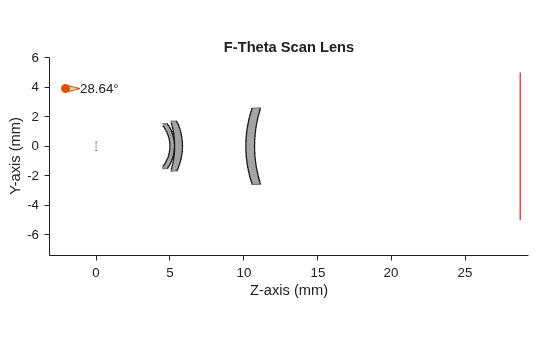
Unlike conventional camera lenses which follow , an f-theta scan lens is designed so that -- image height is directly proportional to the input beam angle. This linear mapping ensures constant scan speed across the image plane, which is critical for uniform laser etching. The lens places its entrance pupil ahead of the first element, providing a physical location for the galvo mirror to sit so that the scan pivot coincides with the pupil plane.
Create a three-element f-theta lens from the Laikin prescription [1] by using the createFThetaLens helper function, included in the supporting project file attached to this example. Visualize the lens system in 2-D by using the view2d function.
opsysFTheta = createFThetaLens;
view2d(opsysFTheta,Parent=figure);
Verify F-Theta Relationship
To illustrate the f-theta property, place a galvo mirror at the entrance pupil and sweep its tilt angle by using the sweepMirrorAngle helper function, included in the supporting project file attached to this example. The reflected beam angle is twice the mirror tilt, so a +/-7 degree mirror sweep directs the beam at +/-14 degrees into the lens, within its 14.3 degree half field of view. The chief ray hit position on the image plane varies linearly with mirror angle, confirming .
angles = -7:2:7;
[hitPos,angles] = sweepMirrorAngle(opsysFTheta,angles);
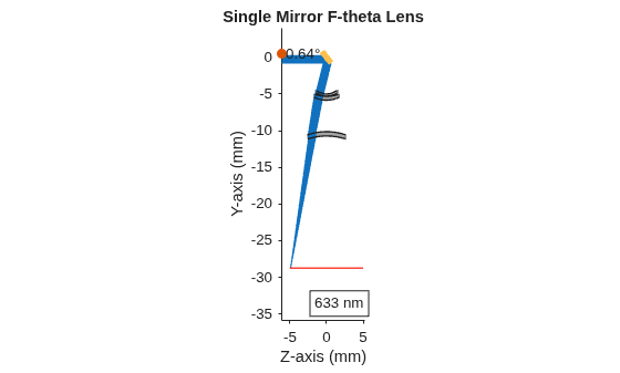
Plot the chief ray hit position versus mirror scan angle to confirm linearity.
figure
plot(angles,hitPos,"o-",LineWidth=1.5)
xlabel("Mirror Scan Angle [deg]")
ylabel("Image Plane Hit Position [mm]")
title("F-Theta Linearity: Image Height vs. Input Angle")
grid on
![Figure contains an axes object. The axes object with title F-Theta Linearity: Image Height vs. Input Angle, xlabel Mirror Scan Angle [deg], ylabel Image Plane Hit Position [mm] contains an object of type line.](../examples/optics/ModelDynamicOpticalSystemsWithScanningElementsExample_03.png)
Quantify Lens Distortion
Quantify how closely the lens achieves the ideal mapping compared to the standard of conventional lenses by using the lensDistortion function. The f-theta distortion is near zero across the field, confirming suitability for scanning.
show(lensDistortion(opsysFTheta,Type="FTheta"),Parent=figure);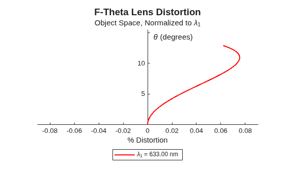
Model Galvo Motor Dynamics
The galvanometer system in this example combines mechanical parameters from the Thorlabs GVS012 dual-axis scanner [2] with motor electrical parameters from the Cambridge Technology 6210H datasheet [3]. Each galvo mirror uses a moving-magnet motor modeled as a DC motor with inertia, viscous damping, and torque constant. The motor dynamics follow:
The parameters used in this example are:
kg m (rotor + mirror inertia; bare rotor is from [3], scaled 100x for mirror load)
N m / (rad/s) (assumed viscous damping)
N m / A (torque constant from [3])
Mirror separation: 14.7 mm center-to-center (derived from [2] CAD drawing)
Mirror aperture: 10 mm diameter (from [2])
In practice, the upstream Galvo X mirror is typically larger than the downstream Galvo Y mirror because it must accommodate the full beam sweep in both axes, which requires a heavier motor. For simplicity, this example uses the same motor parameters for both axes. A proportional-derivative (PD) controller closes the loop around each motor to track the commanded angle.
Tune PD Controller
Each galvo axis uses a Simulink PID Controller block configured in PD mode. The derivative term includes a first-order filter () to avoid amplifying high-frequency noise. The transfer function of the controller is:
You can derive gains by using the PID Tuner app. The gains used in this example are:
You can re-tune these gains by launching the PID Tuner app directly from the PID Controller block dialog box by clicking Tune.
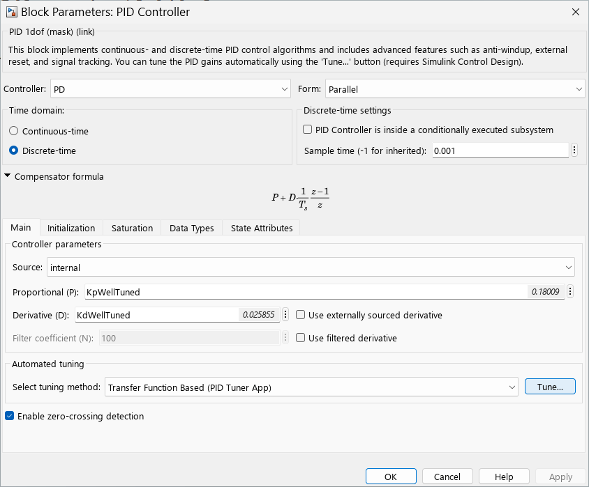
For more details on the tuning workflow, see Automated Tuning of Simulink PID Controller Block.
Create and Visualize Dual-Axis Scanner
The full system combines two galvo mirrors (X then Y) with the f-theta lens. The upstream Galvo X tilts about the Y-axis, controlling X-displacement on the image. The downstream Galvo Y tilts about the X-axis, controlling Y-displacement. Because Galvo Y is downstream of Galvo X, the Y-spot position depends on both mirror angles, creating cross-axis coupling. Assemble the dual-axis scanner by using the createDualAxisFThetaScanner helper function, included in the supporting project file attached to this example. Create a hexapolar sampling grid using the samplingGrid object, and trace rays through the scanner by using the traceRays function.
opsysScanner = createDualAxisFThetaScanner;
sg = samplingGrid("Hexapolar");
rb = traceRays(opsysScanner,SamplingGrid=sg);
Correct Cross-Axis Coupling with Calibration
In a dual-axis scanner, the upstream mirror's deflection influences the downstream mirror's effect on spot position. The upstream X-axis is uncoupled but has a non-standard angular magnification due to the 3-D fold geometry, which you can correct with a simple scale factor computed by tracing a single calibration ray. The downstream Y-axis exhibits true cross-axis coupling: its hit position depends on the current X-mirror angle.
To compensate for the Y-coupling, construct a calibration lookup table before running the simulation by using the buildCalibrationTable helper function, included in the supporting project file attached to this example. This function sweeps all combinations of mirror angles across the operating range, traces rays for each pair, and records the resulting spot positions on the image plane. It then inverts the forward map to produce a lookup table that, given a specified position, returns the corrected Y-mirror command angle accounting for the coupling. Here, you sweep a 21-by-21 grid of angle pairs.
cal = buildCalibrationTable(21);
Simulate Dual-Axis Laser Scanner
The Simulink model implements closed-loop control of both galvo axes. At each timestep, the F-Theta Scan Lens block traces rays through the full optical system and returns the beam hit position on the image plane. The Etch Pattern Command subsystem generates the commanded etch trajectory.
The controller converts specified image-plane positions, in millimeters, to mirror command angles, in degrees. The controller handles each axis differently:
Upstream X-axis — Uses the analytic conversion factor
pos2AngleScale, derived from the standard f-theta relation and the lens focal length. Because the upstream mirror is uncoupled, this single scale factor is sufficient.Downstream Y-axis — Uses a separate conversion factor
pos2AngleScaleY, computed by ray tracing several Y-only sweeps and averaging the ratio of mirror angle to hit position. The 3-D fold geometry gives the downstream mirror a different angular magnification than the standard f-theta formula predicts.Y-axis cross-coupling correction — Applies the 2-D lookup table built by
buildCalibrationTablein the previous section to correct the Y-mirror command angle. Even with the corrected scale factor, the Y-hit position depends on the current X-mirror angle due to cross-axis coupling, so the lookup maps each specified position to the corrected Y-mirror angle.
When you open the model, the InitFcn callback computes these parameters and stores them in the model workspace. To inspect or modify them, open Modeling, and then Model Explorer, and select the model workspace.
open_system("FThetaLaserEtchDemo")Visualize Signals in Simulation Data Inspector
Opening the model automatically launches the Simulation Data Inspector (SDI). To monitor the etch trajectory in real time during simulation:
In the SDI, expand the Actual Etch record in the signal browser on the left.
Select the Actual X and Actual Y signals to plot the actual beam position.
Expand the Ideal Etch record and select the Ideal X and Ideal Y signals to plot the commanded pattern.
To plot the X-position against the Y-position as a 2-D trajectory, right-click a signal and select Plot against another signal.
Signal selections are session-specific and do not persist when you close the model.
Compare Simulation Results
The Use Calibration Constant block controls whether the Y-axis calibration lookup table is applied. Double-click the block and set its value to 0 to use the uncorrected f-theta formula, or 1 to enable the calibration correction. Run the simulation with each setting to compare the results.
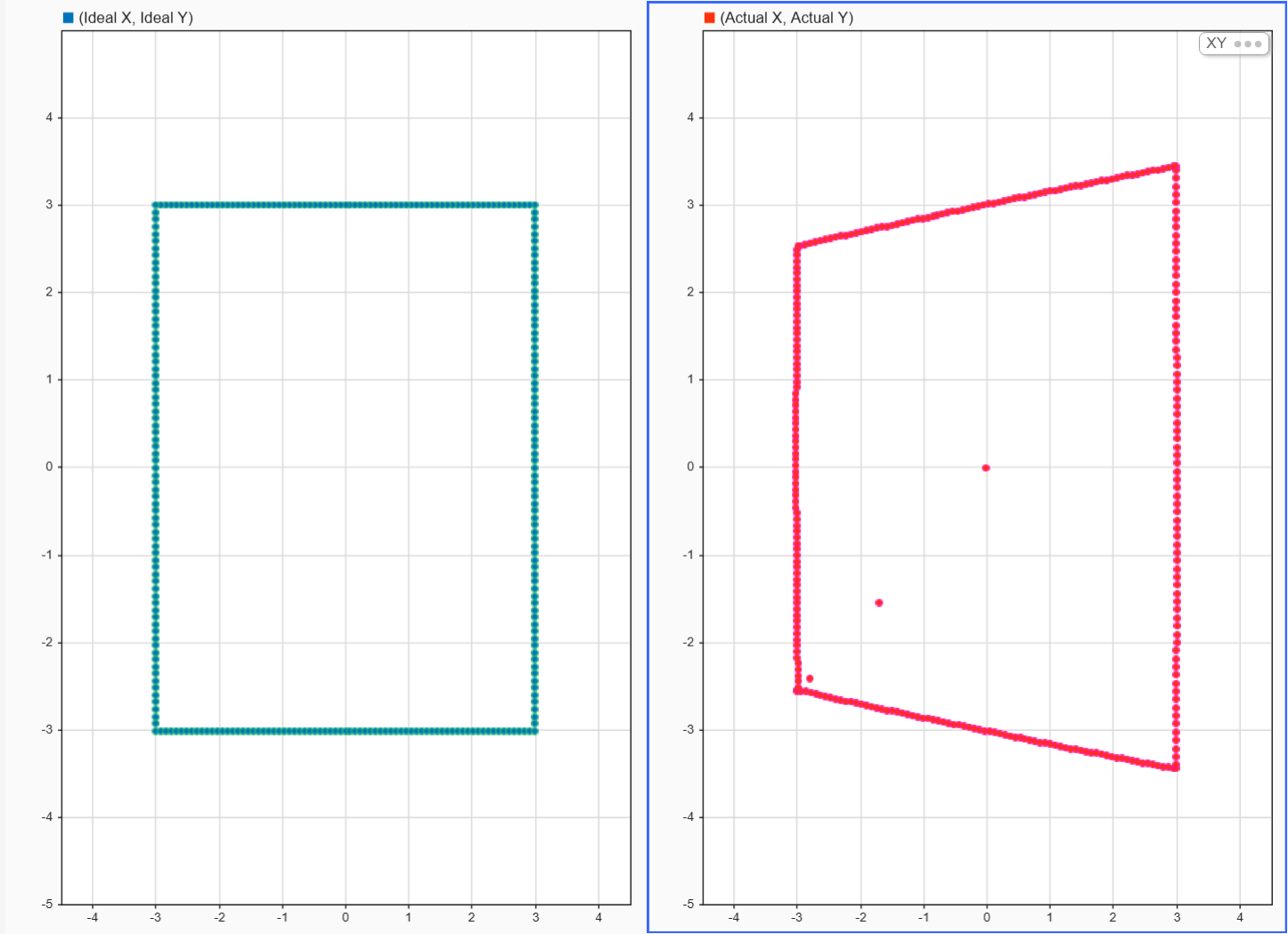
Without calibration, or block value of
0: The X-axis uses the corrected scale factor, but the Y-axis uses the uncorrected f-theta formula without coupling compensation. Cross-axis coupling distorts the Y-positions when X is deflected.
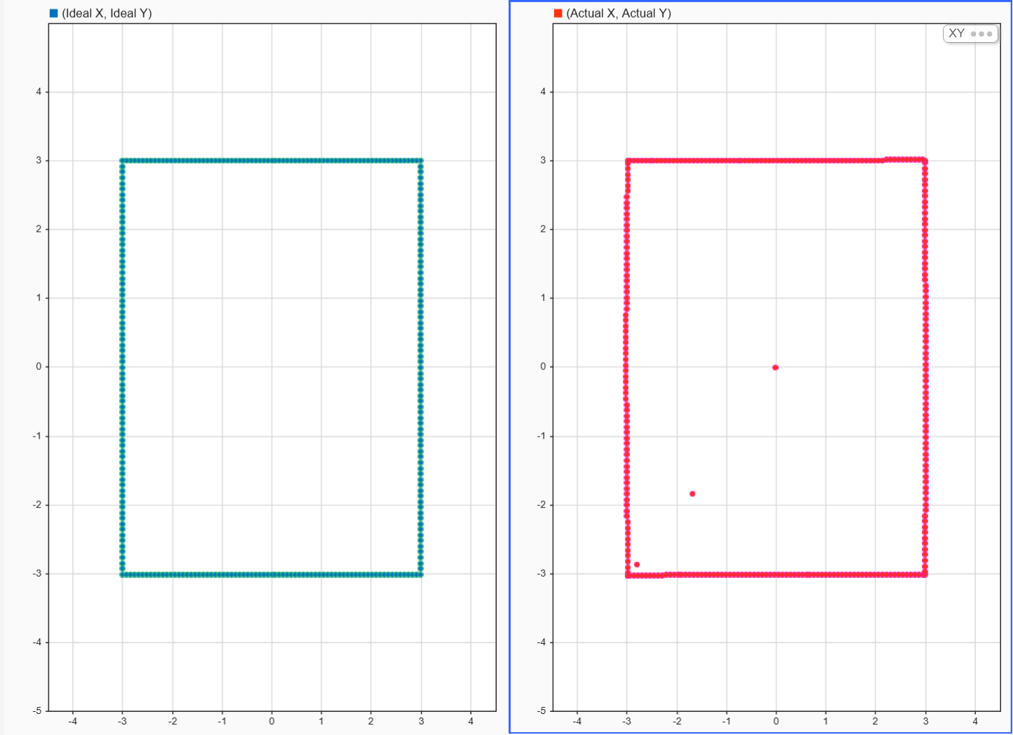
With calibration, or block value of
1: The controller looks up the corrected Y-angle from the pre-computed calibration table, which maps specified positions to the required Y-mirror angle. This corrects for the cross-axis coupling because the lookup accounts for the X-mirror's influence on Y-beam position.
Next Steps
You can supply different etch patterns by modifying the generateSquarePath helper function, included in the supporting project file attached to this example, or replacing it with a custom path generator that returns a structure compatible with the FromWorkspace block. You can also adjust the controller gains (KpWellTuned, KdWellTuned) or motor parameters to observe the effect on tracking performance. To improve correction accuracy at the cost of longer offline computation, specify a larger numPoints value in buildCalibrationTable.
Close Model
Close the Simulink model without saving changes.
close_system("FThetaLaserEtchDemo",0);References
[1] Milton Laikin, Lens Design, 4th ed., CRC Press, 2007, p. 251.
[2] Thorlabs, "GVS012 2D Large Beam (10 mm) Diameter Galvo System," Product Page. https://www.thorlabs.com/item/GVS012 (retrieved June 11, 2026)
[3] Cambridge Technology, "Model 6210H Galvanometer Optical Scanner," 2020. https://www.edmundoptics.com/ViewDocument/manl_11762.pdf

