Simulate Image Using Spatially Variant PSF

R2026b

Since R2026b

This example uses:

Optical Design and Simulation Library for Image Processing Toolbox Optical Design and Simulation Library for Image Processing Toolbox

This example shows how to simulate the image that a lens system forms of a flat scene. The simulation reproduces geometric distortion, lateral chromatic aberration, and spatially varying aberration blur. The approach separates geometry from blur: you warp the scene per wavelength to apply distortion and lateral color, then convolve with chief-ray-centered point spread functions (PSFs) that carry only residual blur [1].

Load and Configure Optical System

Import a wide-angle lens by using the zmximport function. This lens produces pronounced barrel distortion and lateral chromatic aberration toward the field corners. The 440, 510, and 650 nanometer wavelengths represent the blue, green, and red channels, respectively. Attach a 512-by-384 sensor with a 20-micrometer pixel pitch and a 4:3 landscape orientation by using the addImageSensor function.

opsys = zmximport("WideAngleLens.zmx");
opsys.Wavelengths = [440,510,650];
opsys.addImageSensor(PixelSize=20,Resolution=[512,384]);

Create Object Plane

Define the scene as a 210-by-297 mm physical object. Compute the half field of view by using the halfFieldOfView function, then derive the object distance so that the scene height fills 80% of the sensor. Focus the optical system at the computed distance by using the focus method with a fieldPoint object that specifies the on-axis position. Set the circular object plane radius larger than the scene half-diagonal to ensure all backward-traced chief rays intersect the plane.

sceneHeightMM = 210;
sceneWidthMM  = 297;
fillFactor    = 0.8;

halfFOV = halfFieldOfView(opsys);
objectDistance = (sceneHeightMM / 2) / fillFactor / tand(halfFOV);

opsys.focus(FieldPoint=fieldPoint(Position=[0 0 -objectDistance], ...
    ReferenceFrame="Global"));

objectPlaneRadius = max(sceneHeightMM,sceneWidthMM) / fillFactor;
opsys.ObjectPlane = optics.component.ObjectPlane( ...
    Position=[0 0 -objectDistance], ...
    Shape=optics.shape.Circular(objectPlaneRadius));

Prepare Scene

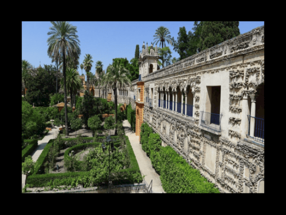
Resize the scene to fill 80% of the sensor rows, preserving the physical aspect ratio for the width in pixels. Center the scene on the output array with zero-padding to represent empty space beyond the object.

outputCols = 512;
outputRows = 384;
pixelSizeMM = 20e-3;

sceneImg = imread("sevilla.jpg");
sceneRowsPx = round(outputRows * fillFactor);
sceneColsPx = round(sceneRowsPx * sceneWidthMM / sceneHeightMM);
sceneImg = imresize(sceneImg,[sceneRowsPx,sceneColsPx]);

padSize = [outputRows,outputCols] - size(sceneImg,[1 2]);
scene = padarray(padarray(sceneImg,floor(padSize/2),0,"pre"), ...
    ceil(padSize/2),0,"post");
imageshow(scene);

Trace Sample Chief Rays

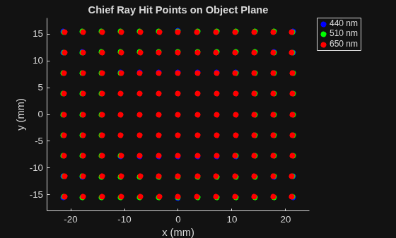
Define a grid of sample field points in the image reference frame by using the fieldPoint function, and trace their chief rays to the object plane by using the traceChiefRay function. The sample grid spans the full sensor so that the distortion map covers every output pixel without extrapolation. Choose an odd number of sample rows for symmetric placement with a center point. Derive the number of columns from the aspect ratio.

numSampleRows = 9;
numSampleCols = 13;
numChannels  = numel(opsys.Wavelengths);

Dx = outputCols / numSampleCols;
Dy = outputRows / numSampleRows;
halfCols = floor(numSampleCols/2);
halfRows = floor(numSampleRows/2);

sampleX = (-halfCols:halfCols) * Dx * pixelSizeMM;
sampleY = (-halfRows:halfRows) * Dy * pixelSizeMM;
[sampleGridX,sampleGridY] = meshgrid(sampleX,sampleY);

sampleFP = fieldPoint(Position=[sampleGridX(:),sampleGridY(:)], ...
    ReferenceFrame="Image");
chiefRays = traceChiefRay(opsys,FieldPoints=sampleFP(:));

numSamples = numSampleRows * numSampleCols;
hitPos = NaN(numSamples,2,numChannels);
for wIdx = 1:numChannels
    rays = chiefRays(:,wIdx);
    valid = arrayfun(@(r) r.RayData.NumRays > 0,rays);
    origins = cell2mat(arrayfun(@(r) r.RayData.Origin(1:2),rays(valid),UniformOutput=false));
    hitPos(valid,:,wIdx) = origins;
end

Visualize Sample Intersection Points

Plot sample intersection positions on the object plane, colored by wavelength. The separation between wavelength markers at each sample position shows lateral chromatic aberration, which increases toward the field edges.

wavelengthColors = [0 0 1; 0 1 0; 1 0 0];
figure
hold on
for wIdx = 1:numChannels
    scatter(hitPos(:,1,wIdx),hitPos(:,2,wIdx), ...
        36,wavelengthColors(wIdx,:),"filled")
end
hold off
xlabel("x (mm)"); ylabel("y (mm)")
title("Chief Ray Intersection Points on Object Plane")
legend(string(opsys.Wavelengths) + " nm",Location="bestoutside")
axis equal padded

Figure contains an axes object. The axes object with title Chief Ray Hit Points on Object Plane, xlabel x (mm), ylabel y (mm) contains 3 objects of type scatter. These objects represent 440 nm, 510 nm, 650 nm.

Create Distortion Displacement Field

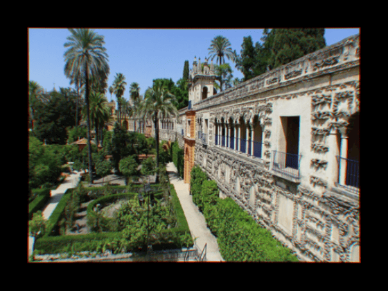
Interpolate the object-plane intersection positions to every output pixel and compute the difference between actual and ideal positions as a pixel displacement field. Fit the paraxial magnification from the first wavelength to define the ideal reference grid. Warp each color channel independently to reproduce geometric distortion and lateral chromatic aberration. The displacement encodes image inversion from negative magnification, which a 180-degree rotation corrects in a later step.

sensorW = outputCols * pixelSizeMM;
sensorH = outputRows * pixelSizeMM;

Compute the paraxial magnification from the first wavelength.

centerIdx = sub2ind([numSampleRows,numSampleCols], ...
    ceil(numSampleRows/2),ceil(numSampleCols/2));
origin = hitPos(centerIdx,:,1);
valid  = ~isnan(hitPos(:,2,1));
magY   = sampleGridY(valid) \ (hitPos(valid,2,1) - origin(2));

Create the object-space reference grid.

maxY = origin(2) + magY * (-sensorH/2);
minY = origin(2) + magY * ( sensorH/2);
xRef = linspace(origin(1) + minY*outputCols/outputRows, ...
                origin(1) + maxY*outputCols/outputRows,outputCols);
yRef = linspace(minY,maxY,outputRows);
[refGridX,refGridY] = meshgrid(xRef,yRef);
pxObj = (xRef(end) - xRef(1)) / (outputCols - 1);
pyObj = (yRef(end) - yRef(1)) / (outputRows - 1);

Create the full sensor grid for interpolation.

[sensorGridX,sensorGridY] = meshgrid(linspace(-sensorW/2,sensorW/2,outputCols), ...
                     linspace(-sensorH/2,sensorH/2,outputRows));

Warp Scene with Distortion

Apply the displacement field to warp each color channel independently, reproducing geometric distortion and lateral chromatic aberration in a single step. Correct the image inversion arising from negative magnification by using the rot90 function.

warpedScene = zeros(outputRows,outputCols,numChannels,"single");
for wIdx = 1:numChannels
    hx = reshape(hitPos(:,1,wIdx),[numSampleRows,numSampleCols]);
    hy = reshape(hitPos(:,2,wIdx),[numSampleRows,numSampleCols]);

    dx = (interp2(sampleGridX,sampleGridY,hx,sensorGridX,sensorGridY) - refGridX) / pxObj;
    dy = (interp2(sampleGridX,sampleGridY,hy,sensorGridX,sensorGridY) - refGridY) / pyObj;

    dx = fillNaN(dx);
    dy = fillNaN(dy);

    % Wavelength order [B G R] maps to channel order [R G B] = [3 2 1]
    ch = numChannels - wIdx + 1;
    warpedScene(:,:,ch) = rot90(single(imwarp(scene(:,:,ch),cat(3,dx,dy))),2);
end
imageshow(warpedScene / 255)

Compute Point Spread Functions

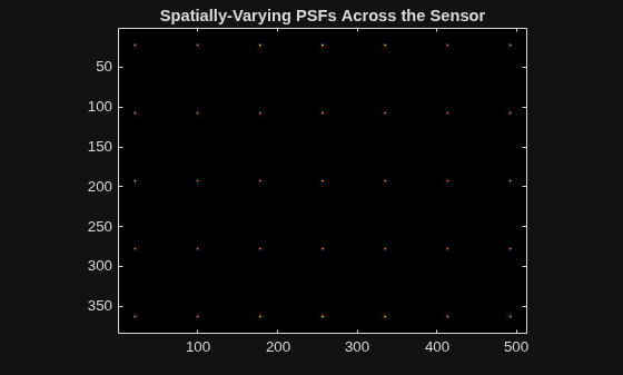
Compute the PSFs on a coarse 5-by-7 sub-grid across the sensor by using the psf function, rather than at every output pixel, because neighboring pixels share nearly the same aberration. Set the Method name-value argument to "Geometric" to trace ray fans through the system. Compute PSFs at half the sensor pixel size for finer aberration detail, then box-average down to sensor scale. For diffraction-accurate blur, set Method to "Huygens" instead. A GPU is recommended when you use "Huygens".

numPsfRows = 5;
numPsfCols = 7;
psfRes     = [64,64];

psfRowIdx = round(linspace(1,numSampleRows,numPsfRows));
psfColIdx = round(linspace(1,numSampleCols,numPsfCols));
psfGridX  = sampleGridX(psfRowIdx,psfColIdx);
psfGridY  = sampleGridY(psfRowIdx,psfColIdx);

[sc,sr] = meshgrid(psfColIdx,psfRowIdx);
psfFP = sampleFP(sub2ind([numSampleRows,numSampleCols],sr(:),sc(:)));
numPsfs = numPsfRows * numPsfCols;

psfStack = zeros(psfRes(2),psfRes(1),numChannels,numPsfs,"single");
for wIdx = 1:numChannels
    result = psf(opsys, ...
        FieldPoints=psfFP, ...
        Method="Geometric", ...
        Wavelengths=opsys.Wavelengths(wIdx), ...
        OutputResolution=psfRes, ...
        PixelSize=10);  % half of 20 um sensor pixel

    hasImg = ~cellfun(@isempty,{result(:).Image});
    % Flip to match image row-down convention for correct convolution
    imgs = flipud(reshape(cat(3,result(hasImg).Image), ...
        [psfRes(2),psfRes(1),1,nnz(hasImg)]));

    ch = numChannels - wIdx + 1;
    psfStack(:,:,ch,hasImg) = imgs;
end

Downsample the PSFs from half-pixel to sensor pixel scale.

psfStack = imresize(psfStack,1/2,"box");

Visualize PSF Variation

Place each colored PSF at its physical sensor position. The PSFs grow larger and more asymmetric toward the field edges, showing how aberration increases with field angle.

psfSize = [size(psfStack,1),size(psfStack,2)];
sensorRef = imref2d([outputRows,outputCols], ...
    [-sensorW/2,sensorW/2],[-sensorH/2,sensorH/2]);
halfPsfW = psfSize(2) * pixelSizeMM / 2;
halfPsfH = psfSize(1) * pixelSizeMM / 2;

splatImage = zeros(outputRows,outputCols,numChannels,"single");
for psfIdx = 1:numPsfs
    cx = psfGridX(psfIdx);
    cy = psfGridY(psfIdx);
    psfRef = imref2d(psfSize,[cx-halfPsfW,cx+halfPsfW],[cy-halfPsfH,cy+halfPsfH]);
    for ch = 1:numChannels
        splatImage(:,:,ch) = splatImage(:,:,ch) + ...
            imwarp(psfStack(:,:,ch,psfIdx),psfRef,affine2d(eye(3)),OutputView=sensorRef);
    end
end
imagesc(rescale(splatImage))
axis image
title("Spatially-Varying PSFs Across the Sensor")

Figure contains an axes object. The axes object with title Spatially-Varying PSFs Across the Sensor contains an object of type image.

Apply Spatially Varying Blur

Build bilinear blending windows for the PSF grid. Each window tapers linearly from 1 at its grid point to 0 at the neighbors. The set of windows sums to one at every pixel, ensuring smooth transitions between PSF regions without gaining or losing image energy. Convolve the windowed scene with the corresponding PSF kernel to produce the final rendered image.

sensorX = sensorGridX(1,:);
sensorY = sensorGridY(:,1);
spacingX = psfGridX(1,2) - psfGridX(1,1);
spacingY = psfGridY(2,1) - psfGridY(1,1);

renderedImage = zeros(outputRows,outputCols,numChannels,"single");
for psfIdx = 1:numPsfs
    [r,c] = ind2sub([numPsfRows,numPsfCols],psfIdx);
    cx = psfGridX(r,c);
    cy = psfGridY(r,c);

    % Tent window = outer product of 1-D triangles
    wx = max(0,1 - abs(sensorX - cx) / spacingX);
    wy = max(0,1 - abs(sensorY - cy) / spacingY);

    % Border extension: fold the phantom neighbor's tent into the edge window
    if c == 1,          wx = wx + max(0,1 - abs(sensorX - cx + spacingX) / spacingX); end
    if c == numPsfCols, wx = wx + max(0,1 - abs(sensorX - cx - spacingX) / spacingX); end
    if r == 1,          wy = wy + max(0,1 - abs(sensorY - cy + spacingY) / spacingY); end
    if r == numPsfRows, wy = wy + max(0,1 - abs(sensorY - cy - spacingY) / spacingY); end

    window = wy * wx;
    for ch = 1:numChannels
        renderedImage(:,:,ch) = renderedImage(:,:,ch) + ...
            conv2(warpedScene(:,:,ch) .* window,psfStack(:,:,ch,psfIdx),"same");
    end
end

renderedImage = renderedImage / max(renderedImage(:));

View Rendered Image

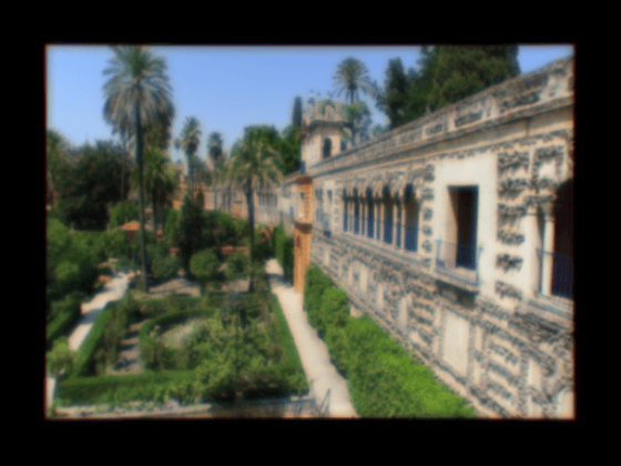
The rendered image shows barrel distortion bending straight lines, lateral chromatic aberration as color fringing toward the field edges, and spatially varying blur that increases toward the corners.

imageshow(renderedImage)

Apply to Other Scenes

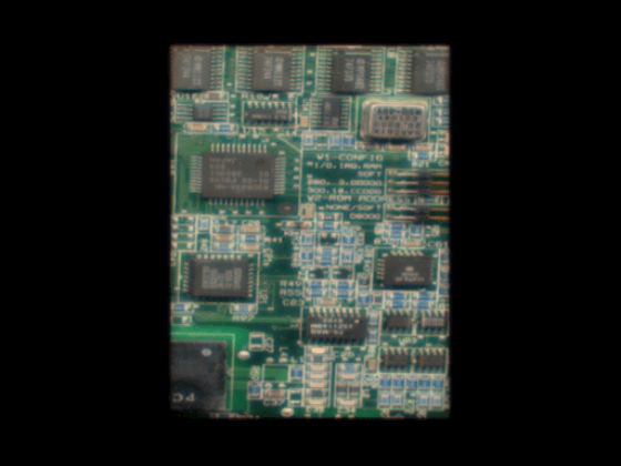
To apply this workflow to other scenes, use the renderImageUsingPSF helper function. This function wraps the full pipeline for any optical system and scene image.

renderedBoard = renderImageUsingPSF(opsys,imread("board.tif"), ...
    Width=210,Height=280,Distance=objectDistance);
imageshow(renderedBoard);

Local Functions

`fillNaN`

Use this function to fill NaN border regions by using pchip interpolation followed by nearest extrapolation.

function out = fillNaN(A)
    out = fillmissing(fillmissing(A,"pchip",2),"pchip",1);
    out = fillmissing(fillmissing(out,"nearest",2),"nearest",1);
end

References

[1] Ho, Chun Jui, Yash Belhe, Samuel Rotenberg, Ravi Ramamoorthi, Tzu-Mao Li, and Nick Antipa. "A Differentiable Wave Optics Model for End-to-End Computational Imaging System Optimization." ICCV (2025).