Aerial Lidar Semantic Segmentation Using RandLANet Deep Learning

Load DALES Data

The DALES data set contains 40 scenes of aerial lidar data. Out of the 40 scenes, 29 scenes are used for training and the remaining 11 scenes are used for testing. Follow the instructions on the DALES website to download the data set to the folder specified by the dataFolder variable. Create folders to store the training and test data.

dataFolder = fullfile(tempdir,"DALES");
trainDataFolder = fullfile(dataFolder,"dales_las","train");
testDataFolder = fullfile(dataFolder,"dales_las","test");

Preview a point cloud from the training data.

lasReader = lasFileReader(fullfile(trainDataFolder,"5080_54435.las"));
[pc,attr] = readPointCloud(lasReader,"Attributes","Classification");
labels = attr.Classification;

% Select only labeled data.
pc = select(pc,labels~=0);
labels = labels(labels~=0);
classNames = ["ground"; ...
    "vegetation"; ...
    "cars"; ...
    "trucks"; ...
    "powerlines"; ...
    "fences"; ...
    "poles"; ...
    "buildings"];
figure
ax = pcshow(pc.Location,labels);
helperLabelColorbar(ax,classNames)
title("Point Cloud with Overlaid Semantic Labels")

Preprocess Training Data

To preprocess the training data, first create a fileDatastore object to collect all the point cloud files in the training data.

fds = fileDatastore(trainDataFolder,"ReadFcn",@lasFileReader);

Each point cloud in the DALES data set covers an area of 500-by-500 meters containing around 10 millions points, processing this many points might slow down network processing. For efficient memory processing, divide the point cloud into small, non-overlapping blocks of size 50-by-50 meters by using the helperTransformData helper function, defined at the end of this example.

Define the block dimensions.

blockSize = [50 50];

Apply the transformation to the training datastore.

ldsTransformed = transform(fds,@(x) helperTransformData(x,blockSize));

Use the helperDatastoreWriteFcn helper function, attached to this example as a supporting file, to save the preprocessed point clouds and semantic labels as PCD and PNG files, respectively. You can set writeFiles to false if your preprocessed training data is already present in the outputFolder.

writeFiles = true;
outputFolder = fullfile(dataFolder,"PreprocessedTrainData");
if writeFiles
    writeall(ldsTransformed,outputFolder,WriteFcn = @helperDatastoreWriteFcn,FolderLayout = "flatten");
end

Processing done for file: 5190_54400.las

Note: Processing can take some time. The code suspends MATLAB® execution until processing is complete.

If you want to rerun the code, you must first use the "clear helperDatastoreWriteFcn" command.

Create Datastore Object for Training

Create a fileDatastore object that reads PCD files by using the pcread function.

pcCropTrainPath = fullfile(outputFolder,"PointCloud");
ldsTrain = fileDatastore(pcCropTrainPath,"ReadFcn",@(x) pcread(x));

Use a pixelLabelDatastore object to store pixel-wise labels from the pixel label images. The object maps each pixel label to a class name and assigns a unique label ID to each class.

% Specify label IDs from 1 to the number of classes.
numClasses = numel(classNames);
labelIDs = 1 : numClasses;
labelCropTrainPath = fullfile(outputFolder,"Labels");
pxdsTrain = pixelLabelDatastore(labelCropTrainPath,classNames,labelIDs);

Use the combine function to combine the point clouds and labels into a single datastore for training.

cds = combine(ldsTrain,pxdsTrain);

Create RandLANet Object

RandLANet is a popular neural network used for semantic segmentation of lidar point clouds. This network uses an encoder-decoder architecture with skip connections. You feed the input to a shared multilayer perceptron layer, followed by four encoding and decoding layers, to learn features for each point. At end, three fully connected layers and a dropout layer associate each point in a 3-D point cloud with a class label, such as car, truck, ground, or vegetation.

This figure shows the architecture of a RandLANet, where:

Each encoding layer randomly downsamples the point cloud, which significantly decreases the point density. To retain the key features of the downsampled point cloud, the network uses a local feature aggregation module on each point.

Each decoding layer upsamples the point feature set through nearest-neighbor interpolation. The network concatenates these upsampled maps with feature maps produced by the encoding layers through skip connections, and applies a shared MLP to the concatenated feature maps.

Use the randlanet function to create a RandLANet segmentation network.

segmenter = randlanet("none",classNames);

Specify Training Options

Use the Adam optimization algorithm to train the network. Use the trainingOptions (Deep Learning Toolbox) function to specify the hyperparameters.

learningRate = 0.01;
numEpochs = 200;
miniBatchSize = 8;
learnRateDropFactor = 0.9886;
executionEnvironment = "auto";

if canUseParallelPool
    dispatchInBackground = true;
else
    dispatchInBackground = false;
end
 
options = trainingOptions("adam", ...
    InitialLearnRate = learningRate, ...
    MaxEpochs = numEpochs, ...
    MiniBatchSize = miniBatchSize, ...
    LearnRateSchedule = "piecewise", ...
    LearnRateDropPeriod = 1,...
    LearnRateDropFactor = learnRateDropFactor, ...
    Plots = "training-progress", ...
    ExecutionEnvironment = executionEnvironment, ...
    dispatchInBackground = dispatchInBackground, ...
    ResetInputNormalization = false, ...
    CheckpointFrequencyUnit = "epoch", ...
    CheckpointFrequency = 10, ...
    CheckpointPath = tempdir, ...
    BatchNormalizationStatistics="moving");

Note: Reduce or increase the miniBatchSize value to control memory usage when training.

Train Model

Use the trainRandlanet function to train the RandLANet segmentation network, set the doTraining argument to true. Otherwise, load a pretrained segmentation network. To train the network, you can use a CPU or GPU. Using a GPU requires Parallel Computing Toolbox™ and a CUDA® enabled NVIDIA® GPU. For more information, see GPU Computing Requirements (Parallel Computing Toolbox).

doTraining = false;
if doTraining
    segmenter = trainRandlanet(cds,segmenter,options);
else
    segmenter = randlanet("dales");
end

Segment Aerial Point Cloud

Create a fileDatastore object to read multiple test point clouds. For demonstration purpose, we are reading a single point cloud.

fdsTest = fileDatastore(fullfile(testDataFolder,"5080_54470.las"),"ReadFcn",@lasFileReader);

Apply the similar transformation used on training data, to the test data:

ldsTestTransformed = transform(fdsTest,@(x) helperTransformData(x,blockSize));

Read all blocks of the test point cloud. Notice X contain pointCloud objects and corresponding labels for all the blocks of the test point cloud.

X = read(ldsTestTransformed);

Create pointCloud object containing array of block of pointClouds of size Mx1. Notice segmentObjects only take pointCloud array of size Mx1 as input.

ptCloudArray = vertcat(X{:,1});

Using segmentObjects function, perform inference to compute prediction labels.

[labels,scores] = segmentObjects(segmenter,ptCloudArray);

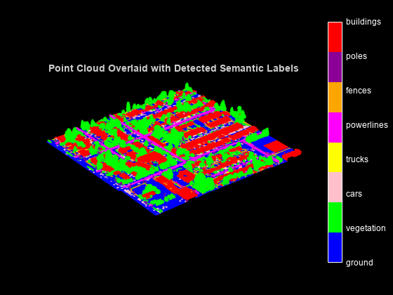
Display the predictions on the point cloud.

% Concatenate blocks of point cloud.
pc = pccat(ptCloudArray);

% Concatenate corresponding labels of blocks of point cloud.
labelsDensePred = vertcat(labels{:});

% Convert labels from categorical to numeric for display.
labelsDensePred = single(categorical(labelsDensePred,classNames,cellstr(string(1:numClasses))));
figure
ax = pcshow(pc.Location,labelsDensePred);
axis off
helperLabelColorbar(ax,classNames)
title("Point Cloud Overlaid with Detected Semantic Labels")

Evaluate Network

To perform evaluation on the test data, get the labels from the test point cloud. Use the predicted labels you computed and are stored in labelsDensePred.

Extract the ground truth labels.

labelsDenseTarget = vertcat(X{:,2});

Use the evaluateSemanticSegmentation function to compute the semantic segmentation metrics from the test set results.

confusionMatrix = segmentationConfusionMatrix(double(labelsDensePred), ...
    double(labelsDenseTarget),Classes = 1:numClasses);
metrics = evaluateSemanticSegmentation({confusionMatrix},classNames,Verbose = false);

You can measure the amount of overlap per class using the intersection-over-union (IoU) metric.

The evaluateSemanticSegmentation function returns metrics for the entire data set, for individual classes, and for each test image. To see the metrics at the data set level, inspect the metrics.DataSetMetrics property.

metrics.DataSetMetrics

ans=1×4 table
    GlobalAccuracy    MeanAccuracy    MeanIoU    WeightedIoU
    ______________    ____________    _______    ___________

       0.95783          0.85172       0.70197      0.92355  

The data set metrics provide a high-level overview of network performance. To see the impact each class has on the overall performance, view the metrics for each class by inspecting the metrics.ClassMetrics property.

metrics.ClassMetrics

ans=8×2 table
                  Accuracy      IoU  
                  ________    _______

    ground        0.97692     0.95547
    vegetation    0.90972     0.89308
    cars          0.95455     0.72914
    trucks        0.34194     0.21973
    powerlines    0.90057     0.86226
    fences        0.89055     0.48276
    poles          0.8624     0.55633
    buildings     0.97709     0.91698

Supporting Functions

The helperTransformData function applies these transformations to the data:

function out = helperTransformData(lasReader,blocksize)

[ptCloud,attr] = readPointCloud(lasReader,"Attributes","Classification");
labels = attr.Classification;

% Select only labeled data.
ptCloud = select(ptCloud,labels~=0);
labels = labels(labels~=0);

% Block the input point cloud.
numGridsX = round((diff(ptCloud.XLimits)+eps)/blocksize(1));
numGridsY = round((diff(ptCloud.YLimits)+eps)/blocksize(2));
[~,~,~,indx,indy] = histcounts2(ptCloud.Location(:,1),ptCloud.Location(:,2), ...
    [numGridsX, numGridsY],XBinLimits = ptCloud.XLimits, YBinLimits = ptCloud.YLimits);
ind = sub2ind([numGridsX, numGridsY],indx,indy);

out = cell(numGridsX*numGridsY,2);

    for num = 1:numGridsX*numGridsY
        idx = ind == num;

        if(any(idx))
            out{num,1} = select(ptCloud,idx);
            out{num,2} = labels(idx);
        end
    end

end

References

[1] Hu, Qingyong, Bo Yang, Linhai Xie, Stefano Rosa, Yulan Guo, Zhihua Wang, Niki Trigoni, and Andrew Markham. “RandLA-Net: Efficient Semantic Segmentation of Large-Scale Point Clouds.” In 2020 IEEE/CVF Conference on Computer Vision and Pattern Recognition (CVPR), 11105–14. Seattle, WA, USA: IEEE, 2020. https://doi.org/10.1109/CVPR42600.2020.01112.

[2] Varney, Nina, Vijayan K. Asari, and Quinn Graehling. “DALES: A Large-Scale Aerial LiDAR Data Set for Semantic Segmentation.” In 2020 IEEE/CVF Conference on Computer Vision and Pattern Recognition Workshops (CVPRW), 717–26. Seattle, WA, USA: IEEE, 2020. https://doi.org/10.1109/CVPRW50498.2020.00101.