Extract Individual Tree Attributes and Forest Metrics from Aerial Lidar Data
This example shows how to extract individual tree attributes and forest metrics from aerial lidar data.
Forest study and applications increasingly use high-density lidar data obtained from airborne laser scanning systems. This data enables measurement of both individual tree attributes and broader forest metrics.
This example uses input point cloud data from a LAZ file, captured by an airborne lidar system. You first segment the point cloud data into ground and vegetation points. Then, you segment vegetation points into distinct trees and extract individual tree attributes. Finally, you compute forest metrics using both the ground and vegetation points. This figure provides an overview of the process.

Load and Visualize Data
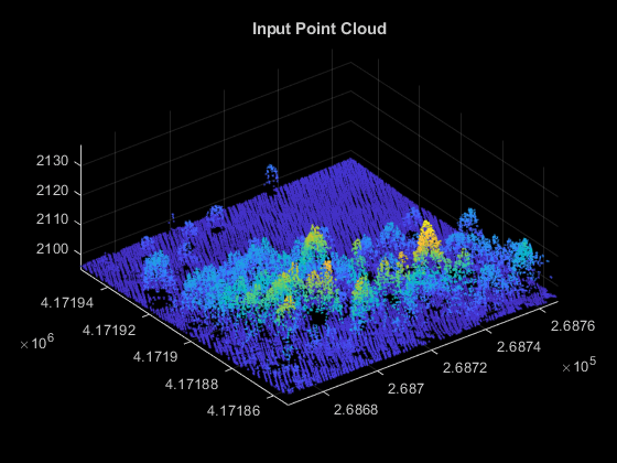
Unzip forestData.zip to a temporary directory and load the point cloud data from the LAZ file, forestData.laz, into the MATLAB® workspace. The data is obtained from the Open Topography Dataset [1]. The point cloud primarily contains ground and vegetation points. Load the point cloud data into the workspace using the readPointCloud function of the lasFileReader object. Visualize the point cloud using the pcshow function.
dataFolder = fullfile(tempdir,"forestData",filesep);
dataFile = dataFolder + "forestData.laz";
% Check whether the folder and data file already exist or not
folderExists = exist(dataFolder,"dir");
fileExists = exist(dataFile,"file");
% Create a new folder if it doesn't exist
if ~folderExists
    mkdir(dataFolder);
end
% Extract aerial data file if it doesn't exist
if ~fileExists
    unzip("forestData.zip",dataFolder);
end
% Read LAZ data from file
lasReader = lasFileReader(dataFile);
% Read point cloud along with corresponding scan angle information
[ptCloud,pointAttributes] = readPointCloud(lasReader,"Attributes","ScanAngle");
% Visualize the input point cloud
hFigInput = figure;
axInput = axes("Parent",hFigInput,"Color",[0 0 0]);
pcshow(ptCloud.Location,"Parent",axInput);
title(axInput,"Input Point Cloud");
Segment Ground
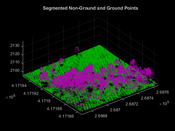
Ground segmentation is a preprocessing step to isolate the vegetation data for extracting forest metrics. Segment the data loaded from the LAZ file into ground and nonground points using the segmentGroundSMRF function.
% Segment Ground and extract non-ground and ground points
groundPtsIdx = segmentGroundSMRF(ptCloud);
nonGroundPtCloud = select(ptCloud,~groundPtsIdx);
groundPtCloud = select(ptCloud,groundPtsIdx);
% Visualize non-ground and ground points in magenta and green, respectively
hFigSegment = figure;
axSegment = axes("Parent",hFigSegment,"Color",[0 0 0]);
pcshowpair(nonGroundPtCloud,groundPtCloud,"Parent",axSegment);
title(axSegment,"Segmented Non-Ground and Ground Points");
Normalize the Elevation
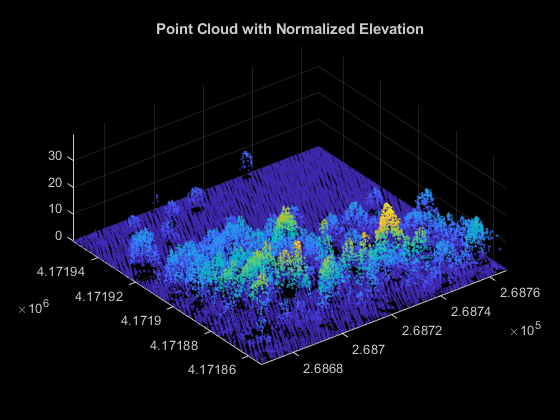
Normalize elevation to remove terrain effects and accurately identify tree heights. Use these normalized points to compute tree attributes and forest metrics. These are the steps for elevation normalization.
Eliminate duplicate points along the x- and y-axes, if any, by using the
groupsummaryfunction.Create an interpolant using the
scatteredInterpolantobject, to estimate ground at each point in the point cloud data.Normalize the elevation of each point by subtracting the interpolated ground elevation from the original elevation.
groundPoints = groundPtCloud.Location;
% Eliminate duplicate points along x- and y-axes
[uniqueZ,uniqueXY] = groupsummary(groundPoints(:,3),groundPoints(:,1:2),@mean);
uniqueXY = [uniqueXY{:}];
% Create interpolant and use it to estimate ground elevation at each point
F = scatteredInterpolant(double(uniqueXY),double(uniqueZ),"natural");
estElevation = F(double(ptCloud.Location(:,1)),double(ptCloud.Location(:,2)));
% Normalize elevation by ground
normalizedPoints = ptCloud.Location;
normalizedPoints(:,3) = normalizedPoints(:,3) - estElevation;
% Visualize normalized points
hFigElevation = figure;
axElevation = axes("Parent",hFigElevation,"Color",[0 0 0]);
pcshow(normalizedPoints,"Parent",axElevation);
title(axElevation,"Point Cloud with Normalized Elevation");
Generate Canopy Height Model (CHM)
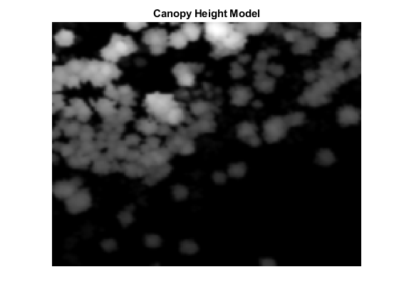
Canopy height models (CHMs) are raster representations of the height of trees, buildings, and other structures above the ground topography. Use a CHM as an input for tree detection and segmentation. Generate the CHM from your normalized elevation values using the pc2dem function.
% Set grid size to 0.5 meters per pixel
gridRes = 0.5;
% Generate CHM
canopyModel = pc2dem(pointCloud(normalizedPoints),gridRes,CornerFillMethod="max");
% Clip invalid and negative CHM values to zero
canopyModel(isnan(canopyModel) | canopyModel<0) = 0;
% Perform gaussian smoothing to remove noise effects
H = fspecial("gaussian",[5 5],1);
canopyModel = imfilter(canopyModel,H,"replicate","same");
% Visualize CHM
hFigCHM = figure;
axCHM = axes("Parent",hFigCHM);
imagesc(canopyModel,"Parent",axCHM);
title(axCHM,"Canopy Height Model");
axis(axCHM,"off");
colormap(axCHM,"gray");
Detect Tree Tops
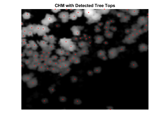
Detect tree tops using the helperDetectTreeTops helper function, attached to this example as a supporting file. The helper function detects tree tops by finding the local maxima within variable window sizes [2] in a CHM. For tree top detection, the helper function considers only points with a normalized height greater than minTreeHeight.
% Set minTreeHeight to 5 m
minTreeHeight = 5;
% Detect tree tops
[treeTopRowId,treeTopColId] = helperDetectTreeTops(canopyModel,gridRes,minTreeHeight);
% Visualize treetops
hFigTreeTops = figure;
axTreeTops = axes("Parent",hFigTreeTops);
imagesc(canopyModel,"Parent",axTreeTops);
hold(axTreeTops,"on");
plot(treeTopColId,treeTopRowId,"rx","MarkerSize",3,"Parent",axTreeTops);
hold(axTreeTops,"off");
title(axTreeTops,"CHM with Detected Tree Tops");
axis(axTreeTops,"off");
colormap(axTreeTops,"gray");
Segment Individual Trees
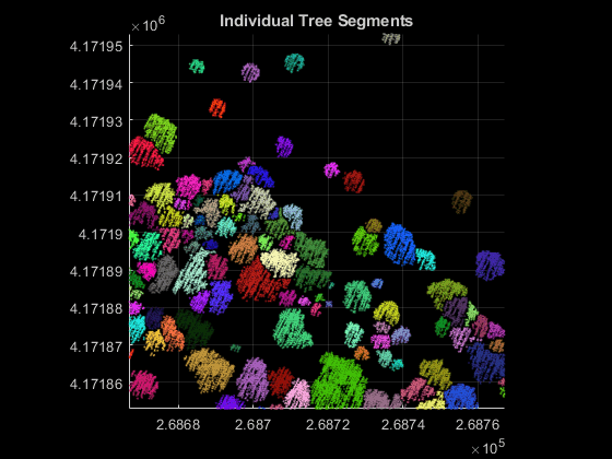
Segment individual trees using the helperSegmentTrees helper function, attached to this example as a supporting file. The helper function utilizes marker-controlled watershed segmentation [3] to segment individual trees. First, the function creates a binary marker image with tree top locations indicated by a value of 1. Then, function filters the CHM complement by minima imposition to remove minima that are not tree tops. The function then performs watershed segmentation on the filtered CHM complement to segment individual trees. After segmentation, visualize the individual tree segments.
% Segment individual trees
label2D = helperSegmentTrees(canopyModel,treeTopRowId,treeTopColId,minTreeHeight);
% Identify row and column id of each point in label2D and transfer labels
% to each point
rowId = ceil((ptCloud.Location(:,2) - ptCloud.YLimits(1))/gridRes) + 1;
colId = ceil((ptCloud.Location(:,1) - ptCloud.XLimits(1))/gridRes) + 1;
ind = sub2ind(size(label2D),rowId,colId);
label3D = label2D(ind);
% Extract valid labels and corresponding points
validSegIds = label3D ~= 0;
ptVeg = select(ptCloud,validSegIds);
veglabel3D = label3D(validSegIds);
% Assign color to each label
numColors = max(veglabel3D);
colorMap = randi([0 255],numColors,3)/255;
labelColors = label2rgb(veglabel3D,colorMap,OutputFormat="triplets");
% Visualize tree segments
hFigTrees = figure;
axTrees = axes("Parent",hFigTrees,"Color",[0 0 0]);
pcshow(ptVeg.Location,labelColors,"Parent",axTrees);
title(axTrees,"Individual Tree Segments");
view(axTrees,2);
Extract Tree Attributes
Extract individual tree attributes using the helperExtractTreeMetrics helper function, attached to this example as a supporting file. First, the function identifies points belonging to individual trees from labels. Then, the function extracts tree attributes such as tree apex location along the x- and y-axes, approximate tree height, tree crown diameter, and area. The helper function returns the attributes as a table, where each row represents the attributes of an individual tree.
% Extract tree attributes
treeMetrics = helperExtractTreeMetrics(normalizedPoints,label3D);
% Display first 5 tree segments metrics
disp(head(treeMetrics,5));
    TreeId    NumPoints    TreeApexLocX    TreeApexLocY    TreeHeight    CrownDiameter    CrownArea
    ______    _________    ____________    ____________    __________    _____________    _________

      1          374        2.6867e+05      4.1719e+06       29.512          7.378          42.753
      2           22        2.6867e+05      4.1719e+06       21.475         0.9905         0.77055
      3          350        2.6867e+05      4.1719e+06       24.216         6.9822          38.289
      4           53        2.6867e+05      4.1719e+06       19.509         3.1956          8.0204
      5          117        2.6867e+05      4.1719e+06       19.399         4.0265          12.733
Extract Forest Metrics
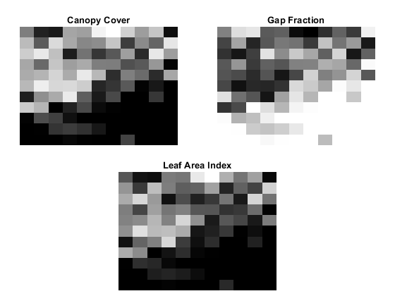
Extract forest metrics from the normalized points using the helperExtractForestMetrics helper function, attached to this example as a supporting file. The helper function first divides the point cloud into grids based on the provided gridSize, and then calculates the forest metrics. Use normalized points instead of raw ground and vegetation points to ensure that metrics are computed based on actual tree height, free from terrain-induced distortions The helper function assumes that all points with a normalized height lower than cutoffHeight are ground and the remaining points are vegetation. Compute these forest metrics.
Canopy Cover (CC) — Canopy cover [4] is the proportion of the forest covered by the vertical projection of the tree crowns. Calculate it as the ratio of vegetation returns relative to the total number of returns.
Gap fraction (GF) — Gap fraction [5] is the probability of a ray of light passing through the canopy without encountering foliage or other plant elements. Calculate it as the ratio of ground returns relative to the total number of returns.
Leaf area index (LAI) — Leaf area index [5] is the amount of one-sided leaf area per unit of ground area. The LAI value is calculated using the equation , where
angis the average scan angle,GFis the gap fraction, andkis the extinction coefficient, which is closely related to the leaf-angle distribution.
% Set grid size to 10 meters per pixel and cutOffHeight to 2 meters
gridSize = 10;
cutOffHeight = 2;
leafAngDistribution = 0.5;
% Extract forest metrics
[canopyCover,gapFraction,leafAreaIndex] = helperExtractForestMetrics(normalizedPoints, ...
    pointAttributes.ScanAngle,gridSize,cutOffHeight,leafAngDistribution);
% Visualize forest metrics
hForestMetrics = figure;
axCC = subplot(2,2,1,"Parent",hForestMetrics);
axCC.Position = [0.05 0.51 0.4 0.4];
imagesc(canopyCover,"Parent",axCC);
title(axCC,"Canopy Cover");
axis(axCC,"off");
colormap(axCC,"gray");
axGF = subplot(2,2,2,"Parent",hForestMetrics);
axGF.Position = [0.55 0.51 0.4 0.4];
imagesc(gapFraction,"Parent",axGF);
title(axGF,"Gap Fraction");
axis(axGF,"off");
colormap(axGF,"gray");
axLAI = subplot(2,2,[3 4],"Parent",hForestMetrics);
axLAI.Position = [0.3 0.02 0.4 0.4];
imagesc(leafAreaIndex,"Parent",axLAI);
title(axLAI,"Leaf Area Index");
axis(axLAI,"off");
colormap(axLAI,"gray");
References
[1] Thompson, S. Illilouette Creek Basin Lidar Survey, Yosemite Valley, CA 2018. National Center for Airborne Laser Mapping (NCALM). Distributed by OpenTopography. https://doi.org/10.5069/G96M351N. Accessed: 2021-05-14
[2] Pitkänen, J., M. Maltamo, J. Hyyppä, and X. Yu. "Adaptive Methods for Individual Tree Detection on Airborne Laser Based Canopy Height Model." International Archives of Photogrammetry, Remote Sensing and Spatial Information Sciences 36, no. 8 (January 2004): 187–91.
[3] Chen, Qi, Dennis Baldocchi, Peng Gong, and Maggi Kelly. “Isolating Individual Trees in a Savanna Woodland Using Small Footprint Lidar Data.” Photogrammetric Engineering & Remote Sensing 72, no. 8 (August 1, 2006): 923–32. https://doi.org/10.14358/PERS.72.8.923.
[4] Ma, Qin, Yanjun Su, and Qinghua Guo. "Comparison of Canopy Cover Estimations From Airborne LiDAR, Aerial Imagery, and Satellite Imagery." IEEE Journal of Selected Topics in Applied Earth Observations and Remote Sensing 10, no. 9 (September 2017): 4225–36. https://doi.org/10.1109/JSTARS.2017.2711482.
[5] Richardson, Jeffrey J., L. Monika Moskal, and Soo-Hyung Kim. "Modeling Approaches to Estimate Effective Leaf Area Index from Aerial Discrete-Return LIDAR." Agricultural and Forest Meteorology 149, no. 6–7 (June 2009): 1152–60. https://doi.org/10.1016/j.agrformet.2009.02.007.
See Also
lasFileReader | readPointCloud | segmentGroundSMRF | lidarPointAttributes