Optimize Spark Ignition Engine Calibration Using Statistical Models
Optimization Overview
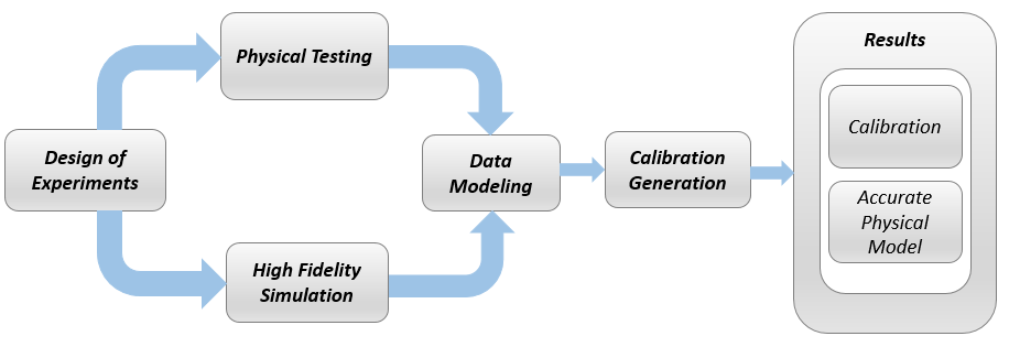
After creating statistical models to fit the data, you can use them in optimizations. You can use the accurate statistical engine model to replace the high-fidelity simulation and run much faster, enabling optimization to generate calibrations in feasible times. You use the statistical models to find the optimal configurations of the engine that meet the constraints.
The statistical models described in Fit Empirical Models to Spark Ignition Engine Calibration Data were used in the next step of model-based-calibration, to create optimized calibration tables.
The aim of the calibration is to maximize torque at specific speed/load values across the engine's operating range, and meet these constraints:
Limit knock (KIT1)
Limit residual fraction
Limit exhaust temperature
Limit calibration table gradients for smoothness.
Turbocharger speed constraints are implicitly included in the boundary model which models the envelope.
The analysis must produce optimal engine calibration tables in speed and load for:
Spark advance ignition timing (SA)
Throttle position % (TPP)
Turbo wastegate area % (WAP)
Air/Fuel Ratio (Lambda: LAM)
Intake cam phase (ICP)
Exhaust cam phase (ECP)
Torque (TQ)
Brake-specific fuel consumption (BSFC)
Boost (MAP)
Exhaust temperature (TEXH)
View Optimization Results
Open MATLAB®. On the Apps tab, in the Automotive group, click MBC Optimization.
In the CAGE Browser home page, in the Case Studies list, open Dual CAM gasoline engine with spark optimized during testing. Alternatively, select File > Open Project and browse to the example file
gasolineOneStage.cag, found inmatlab\toolbox\mbc\mbctraining.In the Processes pane, click Optimization. Observe two optimizations,
Torque_OptimizationandSum_ Torque_Optimization.Why are there two optimizations? To complete the calibration, you need to start with a point optimization to determine optimal values for the cam timings. You use the results of this point optimization to set up a sum optimization to optimize over the drive cycle and meet gradient constraints to keep the tables smooth.
In the Optimization pane, ensure
Torque_Optimizationis selected. In the Objectives pane, observe the description: maximize Torque as a function of ECP, ICP, LOAD and Speed.In the Constraints pane, observe the constraints: the boundary model of Torque, knock, residual fraction, speed and exhaust temperature. If you want to see how these are set up, double-click a constraint and view settings in the Edit Constraint dialog box.
In the Optimization Point Set pane, observe the variable values defining the points at which to run the optimization.
To view the optimization results, in the Optimization pane expand the
Torque_Optimizationnode and selectTorque_Optimization_Output.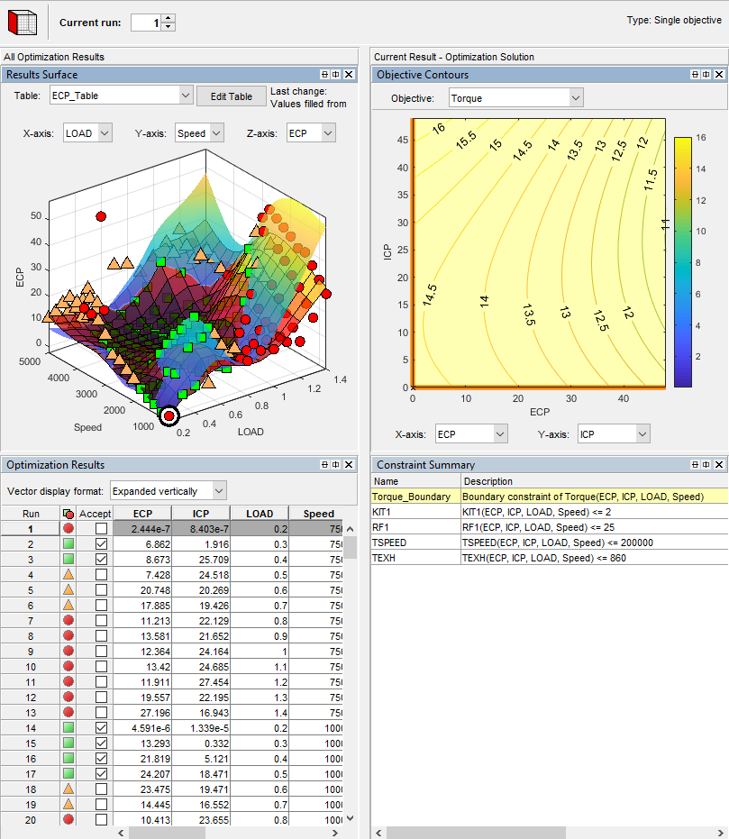
To learn about analyzing optimization results, see View Your Optimization Results.
In the Optimization pane, select
Sum_Torque_Optimizationand compare with the previous point optimization setup.
Set Up Optimization
Learn how to set up this optimization.
To perform an optimization, you need to import the statistical models created in the Model Browser. To see how to import models, in CAGE, select File > Import From Project.
The CAGE Import Tool opens. Here, you can select models to import from a model browser project file or direct from the Model Browser if it is open. However, the toolbox provides an example file with the models already imported, so click Close to close the CAGE Import Tool.
To view the models, click Models in the left Data Objects pane.
You need tables to fill with the results of your optimizations. To see all the tables, select the Tables view.
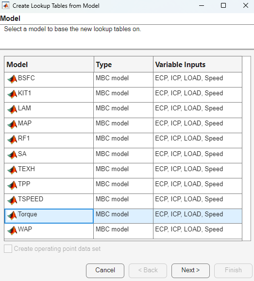
To see how to set up these tables, select Tools > Create Lookup Tables from Model. The Create Lookup Tables from Model wizard appears.
Select the model
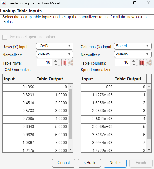
Torqueand click Next.On the next screen you see the controls for specifying the inputs and size of tables. Click the Edit breakpoints buttons to see how to set up row and column values. Click Next.
On the next screen you can set limits on table values. To edit, double-click Table Bounds values.
Click Cancel to avoid creating new unnecessary tables in your example file.
Learn the easiest way to set up an optimization by selecting Tools > Create Optimization from Model.
The Optimization Quick Start Tool start page opens, click Next.
Set Model to
Torque.Observe that the default settings will create a point optimization to minimize
Torque, using 4 free variables, and constrained by a model boundary constraint.To create this example optimization, edit the settings to maximize
Torque. Select onlyECPandICPas Optimization Variables. Click Next.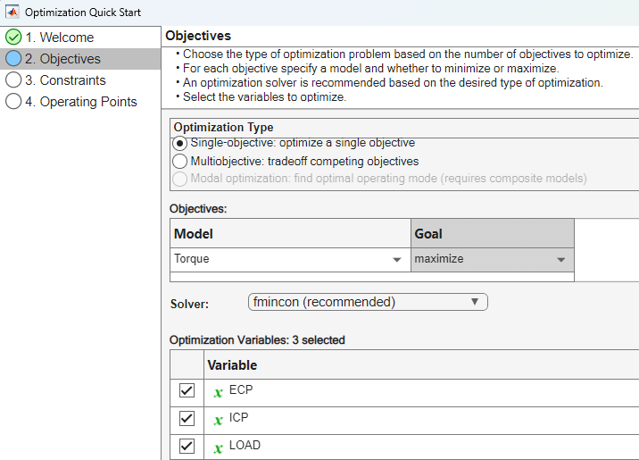
The optimization is constrained by a model boundary constraint. Click Next again.
Set Operating Points to
BreakpointsandTorque_Table(LOAD,Speed). Click Apply to create the optimization.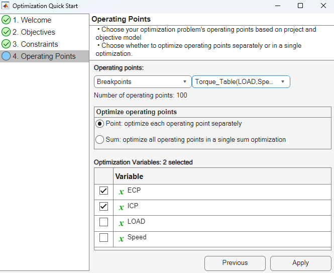
Compare your new optimization with the example
Torque_Optimization. To finish the setup you need to add or import the rest of the constraints. In this case, select Optimization > Constraints > Import Constraints. Import the constraints from theTorque_Optimizationoptimization.To learn how to set up the sum optimization, from the
Torque_Optimization_Outputnode, select Solution > Create Sum Optimization. The toolbox creates a sum optimization for you.Compare your new optimization with the example sum optimization,
Sum_Torque_Optimization. The example shows you need to add the table smoothness constraints to complete the calibration. To see how to set up table gradient constraints, double-click the constraintGradECP.
To learn more about setting up optimizations and constraints, see:
Filling Tables from Optimization Results
CAGE remembers lookup table filling settings. To view how the example tables are filled:
Expand the example sum optimization node
Sum_Torque_Optimizationand select theSum_Torque_Optimization_Outputnode.Select Solution > Fill Lookup Tables to open the Lookup Table Filling from Optimization Results Wizard.
On the first screen, observe all the tables in the CAGE tables to be filled list. Note that the LAM (lambda) table is not filled from the optimization results, because this table was filled from the test data. Click Next.
On the second screen, observe all the tables are matched up with optimization results to fill them with. Click Next.
On the third screen, observe the lookup table filling options. You can either click Finish to fill all the tables, or Cancel to leave the tables untouched. The example tables are already filled with these settings.
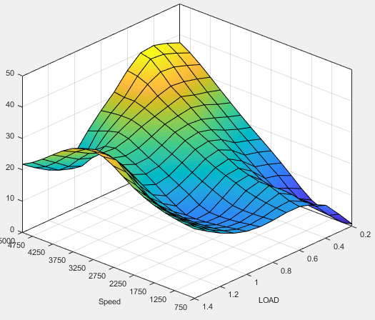
The following plot shows similar calibration results for the ICP table. Observe that the idle region has locked cells to keep the cams parked at 0. If you want to lock values like this, to get smooth filled tables, lock the cells before filling from optimization results.
The following plot shows similar calibration results for the ECP table.
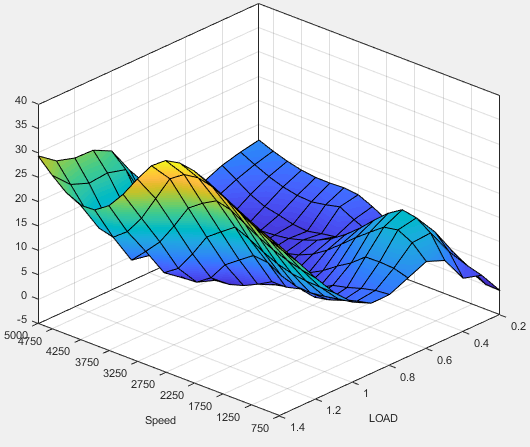
You can examine all the filled tables in the example project.
To learn more about analyzing and using optimization results, see Optimization Analysis.